7 April 2014 by Remco Bouckaert
BEAST 2 stores its internal state occasionally when running an MCMC chain. This means that you can run a chain for a number of samples then resume the chain where it was stopped. This is especially handy when your computer power supply is not very stable or you run BEAST on a cluster that limits the length of jobs.
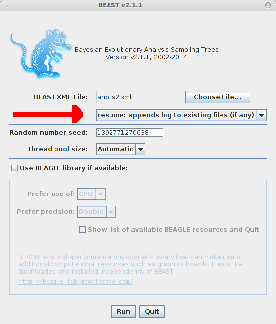
To resume a run, just select the resume option from the BEAST dialog, or if you run from the command line, use the -resume option

Fast model selection/Skipping Burn-in
Disclaimer: this is for exploratory analysis only. For the full analysis running different chains (say 4) till convergence from different random starting points is the recommended way.
Having said this, exploring different models can take a lot of time, choosing different clock models and their configurations, choosing different tree priors, and substitution models with and without gamma heterogeneity and what have you. Exploring all these settings takes time and often it turns out that many models can be dismissed due to their bad performance. However, every time you change settings you have to go through burn-in. If you set of taxa is small, this is no issue, but if you have many taxa and use models with slow convergence, it may pay to use the partial state of a previous run
For example, we set up a Standard analysis in BEAUti, importing the alignment from examples/nexus/anolis.nex, and change the substitution model to HKY, and leave everything at its default settings, then save the file as anolis.xml. So, we start with a simple strict clock analysis with Yule prior, and HKY substitution model without gamma categories or invariant sites. Run BEAST on anolis.xml for a bit, and it produces the file anolis.xml.state that may look something like this:
((((0:0.15218807324699915,(((12:0.07204086917146929,13:0.07204086917146929)45:0.032320490875063,27:0.10436136004653229)35:0.014086879510625344,16:0.11844823955715764)51:0.033739833689841514)48:0.016898052792112206,(22:0.07111803269260457,24:0.07111803269260457)43:0.09796809334650679)55:0.030058453325126883,(((2:0.11202391387224231,28:0.11202391387224231)39:0.053360607716790937,((3:0.05388400742110195,23:0.05388400742110195)30:0.07583538052837979,17:0.12971938794948173)50:0.03566513363955151)41:0.02332777785655904,(19:0.1339032955067472,25:0.1339032955067472)42:0.05480900393884508)53:0.010432279918645954)40:1.2871176295578546E-4,(((((4:0.12883443292345567,20:0.12883443292345567)33:0.018679591712616628,((1:0.09919779884460916,7:0.09919779884460916)44:0.030740336184632705,(11:0.022188644677647536,18:0.022188644677647536)47:0.10774949035159434)46:0.01757588960683043)37:0.01507953828728531,(14:0.1447999403050793,21:0.1447999403050793)49:0.0177936226182783)32:0.013615826070641102,(5:0.10720805090460693,9:0.10720805090460693)29:0.06900133808939178)34:0.01433517128441375,((6:0.09951749852384634,10:0.09951749852384634)54:0.0557955632110991,((8:0.1076629407668736,26:0.1076629407668736)31:0.013630712415594895,15:0.1212936531824685)38:0.03401940855247694)52:0.03523149854346702)36:0.008728730848781563)56:0.0
birthRate.t:anolis[1 1] (-Infinity,Infinity): 7.55654639037806
kappa.s:anolis[1 1] (0.0,Infinity): 3.174302336238077
freqParameter.s:anolis[4 1] (0.0,1.0): 0.27551971155001337 0.26213332703028214 0.11680817105655772 0.34553879036314655
Now, in BEAUti, you can change the site model to use 4 gamma categories and estimate the shape parameter (click check box with ‘estimate’ next to it), — also, change the log file names — and save as anolis2.xml. If you copy anolis.xml.state to anolis2.xml.state and run BEAST on anolis2.xml it will use the end state for the tree, birth rate, kappa and frequency parameters of the anolis.xml run as the starting state of the anolis2.xml run. For the gamma rate, it will use the setting provided in BEAUti.
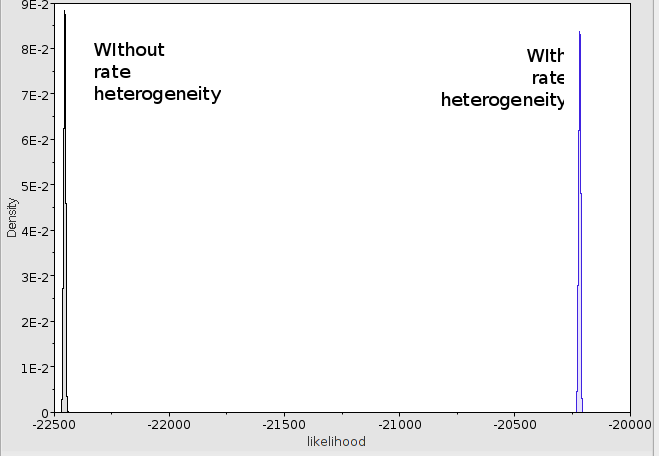
You will notice a rise in posterior from about -22428 to -20328 and a rise in log likelihood from about -22453 to -20345 a whopping 2000 log points improvement. The 95% HDP intervals for the likelihood do not even overlap, so adding gamma
heterogeneity helps in fitting the model considerably in this case and the without heterogeneity model does not be considered any further.

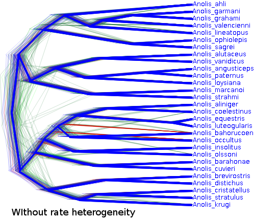
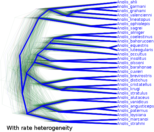
The trees are shaped considerably different as well:


Of course, the anolis dataset with only 29 taxa and 1456 characters in the alignment is just a toy example and there is not such a large gain in speed, but for larger analyses re-using a state can help considerably.
Speeding up MCMC (in some cases)
When the tree is sampled from a bad area — which is almost always is initially, if you start with a random tree — the calculation of the treelikelihood can run into numerical trouble. It will switch to ‘scaling partials’, which can result in a severe performance hit. After a while, the tree can move to an area with higher likelihood and scaling is not required any more. One would think that scaling could be switched off after a while, but that is not always desirable. There are a number of schemes, like NONE, ALWAYS, and DYNAMIC, but we are waiting for the scheme that always works. The code promises this scheme:
KICK_ASS("kickAss"),// should be good, probably still to be discovered
but unfortunately, it is commented out.
One thing you can do to speed up BEAST is switch off scaling, but that may result in zero likelihoods initially. Another thing you can do is run the chain initially with scaling, then stop the chain after a little while and resume the chain. The resumed chain will start without scaling and if it is in a good state, it will not need scaling any more and run a lot faster.
