All posts by rbou019

Simulation studies with BEAST 2

28 April 2014 by Remco Bouckaert

Ever wondered whether the gamma shape that is estimated has any relation to the gamma shape that generated the data? Probably not, but there are many cases where you want to find out whether a model that you use has any relation to the process that generated the data. If so, you probably want to do a simulation study and observe how parameters that generate sequence data have an impact on the parameters of the model that you use to analyse the data.

BEAST has a number of tools that you can use to do a simulation study. Here, we will check what will happen when you change the rate heterogeneity and how it impacts the gamma shape estimate when using the gamma rate heterogeneity model.

Generating an alignment

First of all, we will set up a simulator using the SequenceSimulator class in BEAST. At the time of writing, no GUI is available, so some XML hacking is required.

We will generate a sequence from a 3 taxa fixed tree using the HKY substitution model (kappa=5) and 4 rate categories with gamma shape ranging from 0.2 to 15. The following XML shows how to do this:


        ?
        ?
        ?


			1.0


If you save the XML as simluator.xml you can run it using BEAST, and it will produce a file called gammaShapeSequence.xml containing a sequence alignment with 10000 characters.

Setting up an analysis

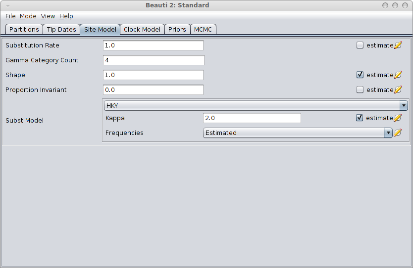
Next step is to create a BEAST MCMC analysis file. The easiest way to do this is using BEAUti. Open BEAUti using the (default) Standard template. Import the alignment from the generated file gammaShapeSequence.xml. Go to the Sitemodel panel, and change the substitution model to HKY. Then, set the number of categories to 4, and click the estimate checkbox next to the shape. The panel should look something like this:

Save the file as analysis.xml. After running the analysis with BEAST, and using tracer to inspect the log file SequenceSimulator.log, tracer could report something like this:

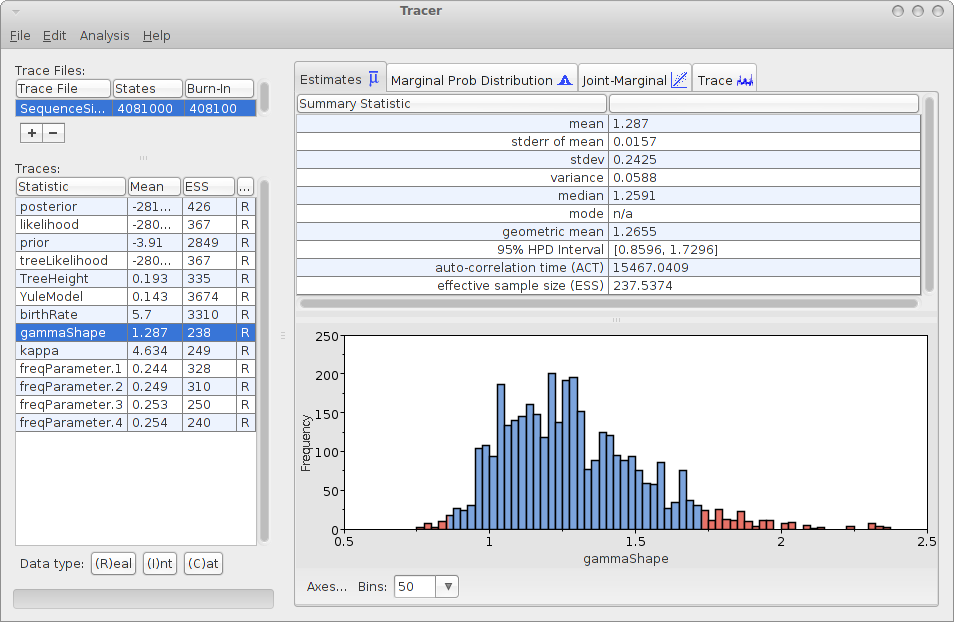
As you can see, the gamma shape is estimated as 1.287 with a 95% HPD Interval of [0.8596, 1.7296], so the original gamma shape value of 1.0 is in the 95% HPD Interval. So, it appears that the gamma shape parameter can be estimated. How about the bias? Perhaps we should run the simulation a few more time and see how it behaves over say 10 independently generated alignments.

Repeating this 10x

To repeat the above — simulate sequences, merge with an analysis, and run the analysis — say 10 times, we can adjust the XML script simply by adding the following:

  • Add an iterations attribute to the run element, setting iterations="10".
  • Add a merge element indicating that the generated alignment should be merged with the XML representing an analysis — it replaces the alignment in a BEAST XML file with the one generated by the SequenceSimulator. Since we just created the file analysis.xml with the kind of analysis we want to run, we can use that file.
  • Note that you can specify more than one merge file, and every template file has its alignment replaced with the same generated alignment. This is handy if you want to find out how model misspecification impacts your estimates.

    The XML should look something like this:


            ?
            ?
            ?


    			1.0


    Save as simulator10.xml in the directory containing analysis.xml and when you run the XML file with BEAST, there should be 10 files generated, named analysis-0.xml, analysis-1.xml, up to analysis-9.xml. You could run the ten XML files with BEAST, but you will quickly find out that every log file has the same name — running each file in its own directory, or renaming log files after running an analysis is quite labourious.

    Fortunately The sequence simulator, before it replaces the alignment in the analysis file, replaces every instance of “$(n)” (dollar followed (n)) by the iteration number. So, if we change the file names of the loggers in the analysis.xml file like so:

    From


    to


    And, from


    to


    It is probably also a good idea to set the chainLength="4000000" in analysis.xml. Rerun BEAST on simluator10.xml.

    Now we can run the 10 simulator files and get log file SequenceSimulator-0.log, SequenceSimulator-1.log, … SequenceSimulator-9.log.

    Analysing the log files can be done with tracer with the 10 log files. For the 10 log files, we can select the combined log, which looks something like this:

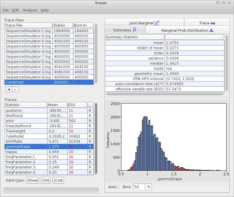
    The mean estimate over 10 runs is 1.0752 with 95% HPD Interval of [0.7423, 1.503], so the gamma shape used for generating the data is close to the mean and it is firmly in the 95% HPD interval.

    Repeating 10x for 21 different gamma shape values

    So, it looks like the gamma shape value can be infered when the value is 1.0. How about other values? To test this, we can change the simulator.xml file for different values of the shape parameter, and run the analysis 10 times for each gamma shape.

    Analysing with LogAnalyser and R

    Doing this for 21 values of the shape parameter gives 210 log files, which become a bit cumbersome to analyse with tracer. If you would have run the same analysis with a different template (e.g. with a GTR model instead of HKY), you get another 210 log files.

    BEAST has a LogAnalyser that produces similar output to tracer in table format. To run it, you can use

    java -cp beast.jar  beast.util.LogAnalyser trace.log

    Running it on one of the trace logs produces output like this:

    ~> java -cp beast.jar beast.util.LogAnalyser SequenceSimulator-9.log
    Loading SequenceSimulator-9.log skipping 400 log lines
    
    |---------|---------|---------|---------|---------|---------|---------|---------|
    *********************************************************************************
    
    Calculating statistics
    
    |---------|---------|---------|---------|---------|---------|---------|---------|
    ********************************************************************************
    
    item            mean     stderr   stddev   median   95%HPDlo 95%HPDup ACT      ESS      geometric-mean 
    posterior       -28426.3 0.104762 1.962981 -28426.0 -28430.0 -28422.9 10256.42 351.0971 NaN     
    likelihood      -28422.3 0.104126 1.814905 -28422.0 -28425.7 -28419.3 11853.12 303.8017 NaN     
    prior           -4.05647 0.01505  0.768483 -3.79066 -5.60204 -3.26877 1381.170 2607.208 NaN     
    treeLikelihood  -28422.3 0.104126 1.814905 -28422.0 -28425.7 -28419.3 11853.12 303.8017 NaN     
    TreeHeight      0.200092 0.000399 0.006715 0.199813 0.187791 0.213805 12723.26 283.0248 0.19998 
    YuleModel       0.009806 0.013149 0.757205 0.290776 -1.48896 0.721453 1085.933 3316.040 NaN     
    birthRate       5.396959 0.054138 3.102894 4.803029 0.51353  11.32685 1096.214 3284.940 4.521489
    gammaShape      1.198491 0.013759 0.195758 1.186229 0.853668 1.591099 17788.98 202.4286 1.183323
    kappa           4.993622 0.017951 0.231987 4.993078 4.55073  5.396354 21561.68 167.0091 4.988256
    freqParameter.1 0.25509  0.000216 0.003752 0.254981 0.248605 0.262504 11883.76 303.0184 0.255063
    freqParameter.2 0.24809  0.000193 0.003549 0.24805  0.241616 0.255487 10634.58 338.6120 0.248064
    freqParameter.3 0.246065 0.00022  0.003662 0.245816 0.239572 0.25322  13036.39 276.2267 0.246038
    freqParameter.4 0.250755 0.000213 0.003567 0.250743 0.244575 0.258267 12875.19 279.6851 0.250729
    

    For this run, the estimated gamma shape is 1.198491 with an ESS of 202.

    By specifying the prefix directive, you can add a column to identify the run by a prefix value. For example, setting -Dprefix=1.0 like so:

    ~> java -Dprefix=1.0 -cp beast.jar beast.util.LogAnalyser SequenceSimulator-9.log
    
    Loading SequenceSimulator-9.log skipping 400 log lines
    
    |---------|---------|---------|---------|---------|---------|---------|---------|
    *********************************************************************************
    
    Calculating statistics
    
    |---------|---------|---------|---------|---------|---------|---------|---------|
    ********************************************************************************
    
    item            prefix mean     stderr   stddev   median   95%HPDlo 95%HPDup ACT      ESS      geometric-mean 
    posterior       1.0 -28426.3 0.104762 1.962981 -28426.0 -28430.0 -28422.9 10256.42 351.0971 NaN     
    likelihood      1.0 -28422.3 0.104126 1.814905 -28422.0 -28425.7 -28419.3 11853.12 303.8017 NaN     
    prior           1.0 -4.05647 0.01505  0.768483 -3.79066 -5.60204 -3.26877 1381.170 2607.208 NaN     
    treeLikelihood  1.0 -28422.3 0.104126 1.814905 -28422.0 -28425.7 -28419.3 11853.12 303.8017 NaN     
    TreeHeight      1.0 0.200092 0.000399 0.006715 0.199813 0.187791 0.213805 12723.26 283.0248 0.19998 
    YuleModel       1.0 0.009806 0.013149 0.757205 0.290776 -1.48896 0.721453 1085.933 3316.040 NaN     
    birthRate       1.0 5.396959 0.054138 3.102894 4.803029 0.51353  11.32685 1096.214 3284.940 4.521489
    gammaShape      1.0 1.198491 0.013759 0.195758 1.186229 0.853668 1.591099 17788.98 202.4286 1.183323
    kappa           1.0 4.993622 0.017951 0.231987 4.993078 4.55073  5.396354 21561.68 167.0091 4.988256
    freqParameter.1 1.0 0.25509  0.000216 0.003752 0.254981 0.248605 0.262504 11883.76 303.0184 0.255063
    freqParameter.2 1.0 0.24809  0.000193 0.003549 0.24805  0.241616 0.255487 10634.58 338.6120 0.248064
    freqParameter.3 1.0 0.246065 0.00022  0.003662 0.245816 0.239572 0.25322  13036.39 276.2267 0.246038
    freqParameter.4 1.0 0.250755 0.000213 0.003567 0.250743 0.244575 0.258267 12875.19 279.6851 0.250729
    

    This makes it easy to have for example an R script to find the estimates associated with a particular value used for generating the data.

    If you specify more than one indicators, for example the iteration number and the shape parameter, just insert them in braces, like so

    ~> java -Dprefix="1.0 9" -cp beast.jar beast.util.LogAnalyser SequenceSimulator-9.log
    

    The output now has two columns, with headers labeled prefix0 prefix1 and column values 9 1.0

    item            prefix0 prefix1 mean     stderr   stddev   median   95%HPDlo 95%HPDup ACT      ESS      geometric-mean 
    posterior       9 1.0 -28426.3 0.104762 1.962981 -28426.0 -28430.0 -28422.9 10256.42 351.0971 NaN     
    likelihood      9 1.0 -28422.3 0.104126 1.814905 -28422.0 -28425.7 -28419.3 11853.12 303.8017 NaN     
    prior           9 1.0 -4.05647 0.01505  0.768483 -3.79066 -5.60204 -3.26877 1381.170 2607.208 NaN     
    treeLikelihood  9 1.0 -28422.3 0.104126 1.814905 -28422.0 -28425.7 -28419.3 11853.12 303.8017 NaN     
    TreeHeight      9 1.0 0.200092 0.000399 0.006715 0.199813 0.187791 0.213805 12723.26 283.0248 0.19998 
    YuleModel       9 1.0 0.009806 0.013149 0.757205 0.290776 -1.48896 0.721453 1085.933 3316.040 NaN     
    birthRate       9 1.0 5.396959 0.054138 3.102894 4.803029 0.51353  11.32685 1096.214 3284.940 4.521489
    gammaShape      9 1.0 1.198491 0.013759 0.195758 1.186229 0.853668 1.591099 17788.98 202.4286 1.183323
    kappa           9 1.0 4.993622 0.017951 0.231987 4.993078 4.55073  5.396354 21561.68 167.0091 4.988256
    freqParameter.1 9 1.0 0.25509  0.000216 0.003752 0.254981 0.248605 0.262504 11883.76 303.0184 0.255063
    freqParameter.2 9 1.0 0.24809  0.000193 0.003549 0.24805  0.241616 0.255487 10634.58 338.6120 0.248064
    freqParameter.3 9 1.0 0.246065 0.00022  0.003662 0.245816 0.239572 0.25322  13036.39 276.2267 0.246038
    freqParameter.4 9 1.0 0.250755 0.000213 0.003567 0.250743 0.244575 0.258267 12875.19 279.6851 0.250729
    

    Using the LogAnalyser, you can create a text file containing the estimates for all logs. Doing this for various values of gamma shape,

    java -Dprefix=0.2 -cp beast.jar beast.util.LogAnalyser SequenceSimulator-0.2.log >> log.dat
    java -Dprefix=0.3 -cp beast.jar beast.util.LogAnalyser SequenceSimulator-0.3.log >> log.dat
    java -Dprefix=0.4 -cp beast.jar beast.util.LogAnalyser SequenceSimulator-0.4.log >> log.dat
    ...
    java -Dprefix=15.0 -cp beast.jar beast.util.LogAnalyser SequenceSimulator-15.log >> log.dat
    

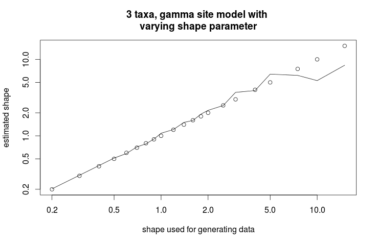
    You can create a log.dat that you can use in R for a plot. In R, we can do the following — assuming we generated alignments with shape parameter values 0.2, 0.3, 0.4, 0.5, 0.6, 0.7, 0.8, 0.9, 1.0, 1.2, 1.4, 1.6, 1.8, 2.0, 2.5, 3.0, 4.0, 5.0, 7.5,10.0, 15.0:

    > x <- read.table("log.dat",header=1)
    > s <- c(0.2, 0.3, 0.4, 0.5, 0.6, 0.7, 0.8, 0.9, 1.0, 1.2, 1.4, 1.6, 1.8, 2.0, 2.5, 3.0, 4.0, 5.0, 7.5,10.0, 15.0)
    > plot(s,s,log="xy",ann=0);
    > lines(s,as.numeric(as.character(x[which(x$item=="gammaShape"),"mean"])))
    > title("3 taxa, gamma site model with nvarying shape parameter", xlab="shape used for generating data", ylab="estimated shape")
    

    This gives the following graph showing the estimate of shape parameter against the value used for simulating the data. Over all, there is a close match, except for large values of the shape parameter.

    BEAST 2 paper is out!

    21 April 2014 by Remco Bouckaert

    The BEAST paper “BEAST 2: A software platform for Bayesian evolutionary analysis” by Remco Bouckaert, Joseph Heled, Denise Kuehnert, Tim Vaughan, Chieh-Hsi Wu, Dong Xie, Marc Suchard, Andrew Rambaut, and Alexei J Drummond is now available from PLOS Computational Biology 10(4), in case you want to cite BEAST 2 (which 3 people already did at the date of publication, according to Google scholar 🙂 ). PLOS Comp Bio is one journal in the series of open access PLOS publications with a knowledgeable editorial board and fast review time and publication process, so there is a lot to commend PLOS Comp Bio.

    However, (disclaimer: the following is my personal opinion/experience and does not necessarily reflect any of those of my co-authors) the publication process left some things to be desired. Previously I published with the Journal of Machine Learning Research, which I would consider the ideal publisher: it is open access, has a high impact factor and there are no fees. Let’s look at some specific issues comparing PLOS and JMLR.

    Cost

    For JMLR, MIT provides the web server, saving few hundred dollars per year it would otherwise cost for commercial web hosting. According to an insider, editor in chief and editorial board are volunteers and webmasters is a student volunteer — note that I never noticed any chance in the lean submission and manuscript management system through the years, the system just works and does not require any development (even though it looks a bit unpolished). Like for most journals, reviewers are unpaid volunteers, so there is not costs involved there. The highest cost involved is a tax accountant, and average cost per paper is estimated at $6.50, covered by donations and MIT.

    PLOS Comp Bio on the other hand charges $2300 per paper to be paid by the authors. Now, JMLR is an extreme example in that it relies on volunteers to a large extend and I appreciate not every journal could be run that way. Also, this is much lower than the more than $5000 ($8 billion revenue for 1.5 million papers) on average commercial publishers receive per paper, but still, it is a significant amount.

    Paper submission

    For JMLR, submitting a paper does not take a lot of effort — it is a one page form that only requires entering all authors on your paper, uploading the pdf paper and a cover letter (if you want to), and entering the title. Apparently, that is all that is required for running a high quality journal for a specialised field. Recommending reviewers is not required, since the editorial board is sufficiently knowledgeable to know the people in the field. If you need to declare conflict of interest, this can be done in the cover letter, and one does not have to go through some hoops like copying some standard phrase in a text field declaring no conflict of interest exists.

    Compare that to submissions to PLOS; there are many HTML pages involved, and lots of information is required — such as conflicts of interests — before one is able to complete a submission. Just for going through the process of submitting a paper and filling in the forms one has to reserve a couple of hours.

    Guidelines

    For JMLR, a Latex style file (jmlr2e.sty) is provided that is easy to use. You prepare your file as any Latex file and have full control over how it looks like.

    JMLR article format instructions are 2866 words when copying the page and counted in Word while PLOS’s is just over 7000 words, more than double that. But that is not all, there are separate guidelines for Latex document, figure and tables, and Supporting information none of which an author should be burdened with, since this is where publishers can add value, but apparently chooses not to.

    Production process

    JMLR author guidelines are short, to the point and contains a 8 point checklist that is helpful in submitting your paper. PLOS just insists that each author has to become an expert in publishing production processes — requiring skills such as converting between graphic file formats, embedding fonts in EPS files, scaling graphics to size, etc. None of these skills are required when using Latex with JMLR — you can just use your favourite file format and stick with that, and submit the Latex output.

    I appreciate that PLOS publishes in different formats, and given the Latex source, it should be able to do so. Unfortunately, that process is broken — it does not convert characters with umlauts properly, and inserted random characters, in the case of the BEAST paper. One would think that these would be issues that should have been fixed by now. The amount of time me and my co-authors wasted on tedious typesetting issues like the above would be zero if we would have published with a system that JMRL provides.

    Most authors that publish with PLOS do not use Latex, so this might be a relatively convenient process for the majority of papers submitted as Word document, but I think there is room for improvement.

    Alternatives

    I am picking out PLOS here because that is where the BEAST paper is published, but there are many other journals that come with a similarly uncomfortable production process.

    Unfortunately, for most bioinformatics papers, JMLR is not an option and it would not have been appropriate for the BEAST paper. I am curious about experience with PeerJ, which appears to offer a smooth interface for submitting papers in Latex. I am not quite sure about the requirements for images though — the author guidelines (a pleasant 3000 word document) still mention the arcane EPS format.

    Programming BEAST without Java

    14 April 2014 by Remco Bouckaert

    If you want to log say a simple function of a parameter or set of parameters, programming a logger in Java is often overkill. A much simpler way is to use some of the scripting functionality that in BEAST. There are a number of options;

  • RPNCalculator which takes expressions in reverse polish notation
  • ExpParser in the MASTER? package, you can use which takes arithmetic expressions
  • Script in the BEASTLabs package, you can use complex arithmetic expressions as well as functions
  • RPNCalculator

    RPNCalculator is the simplest and most primitive of the lot. It takes as input a set of Functions and an expression in reverse Polish notation (RPN). RPN is stack based, and takes arguments first, and whenever an operator is pushed on the stack, it uses the top most positions to execute the operator. So “2 3 +” returns 5, “2 2 2 / /” return 0.5 as does “2 2 2 * /”. Variable names are resolved by the IDs of the arguments. Below, a complete XML fragment


    ExpCalculator

    ExpCalculator can be found in the feast package and allows simple expressions to used as a Function. For example, to calculate the Eucledian distance to the point (20,50), you could use the following:

    20
    50


    There is also a ExpCalculatorDistribution that you can use as a distribution where you can specify an expression to represent to log-density of the distribution. For example — ignoring constants — a normal distribtion could be specified like so:


    which can be used in for example the prior. For more information, see the feast package.

    Script

    To use Script you need to install the BEASTLab package (see the BEAST website for how to install packages).

    With beast.util.Script you can now run complex mathematical expressions like

    3 * sin(a[0]) + log(a[1]) * b 

    where a is a Function with 2 dimensions and b a single values Function. Parameters and Distributions are Functions, so you can use these for your expressions. Since Script is also a Function you can use the result of a Script in another Script.

    Script has an input named x, and every Function and the variable names in the expression must match the ID of the input-value. A complete XML fragment for logging the above expression with two parameters a and b could look something like this:

    1.0 2.0
    3.0


    With Script, you can define complex and recursive functions, for example factorial, like so:

    function fac(x) {
            if (x <= 1) {return 1;}
            return x * fac(x-1);
    }
    
    function f(a) {return fac(a);}
    

    Note that if you specify a scripts instead of an expression, the engine always
    calls function f with arguments of the inputs x in order of appearance. The function specification goes as text inside the element, unlike an expression, which goes inside the expression attribute. An XML fragment logging the factorial of parameter a could look something like this:

    5.0


    	function fac(x) {
    		    if (x <= 1) {return 1;}
    		    return x * fac(x-1);
    	}
    
    	function f(a) {return fac(a);}


    Note that because the text is XML, any XML character (especially '<' and '&') need to be escaped. The <= in the above script must replaced by &lt;=. To prevent this, you can wrap the text in a CDATA block, of which the content is not interpreted as XML but taken as is.

    5.0


    Script syntax

    By default, the Script uses JavaScript syntax for coding expressions and functions. For expressions, the Math scope is used, so any Math-function is available, so the following functions are available: abs(), acos(), asin(), atan(), atan2(), ceil(), cos(), exp(), floor(), log(), max(), min(), pow(), random(), round(), sin(), sqrt(), tan(). A disadvantage is that debugging is awkward to put it mildly. If it does not compile, the ScriptEngine does not offer much clues to where things go wrong.

    You can specify other script engines by setting the engine attribute to one of JavaScript, python, jruby, or groovy and provided the script engine is available in your class path, you can use other syntax for specifying a script (though not for expressions). For example, to use python, you need to include jython in the class path, and set engine='python' on the Script element. A factorial logger could be done like this in python:


    So far, these scripts are rather simple, and can effectively only useable for logging of advanced information. In a later blog, we will look how to use scripts in other situations. But for now happy scripting!

    Checkpointing Tricks

    7 April 2014 by Remco Bouckaert

    BEAST 2 stores its internal state occasionally when running an MCMC chain. This means that you can run a chain for a number of samples then resume the chain where it was stopped. This is especially handy when your computer power supply is not very stable or you run BEAST on a cluster that limits the length of jobs.

    To resume a run, just select the resume option from the BEAST dialog, or if you run from the command line, use the -resume option

    Fast model selection/Skipping Burn-in

    Disclaimer: this is for exploratory analysis only. For the full analysis running different chains (say 4) till convergence from different random starting points is the recommended way.

    Having said this, exploring different models can take a lot of time, choosing different clock models and their configurations, choosing different tree priors, and substitution models with and without gamma heterogeneity and what have you. Exploring all these settings takes time and often it turns out that many models can be dismissed due to their bad performance. However, every time you change settings you have to go through burn-in. If you set of taxa is small, this is no issue, but if you have many taxa and use models with slow convergence, it may pay to use the partial state of a previous run

    For example, we set up a Standard analysis in BEAUti, importing the alignment from examples/nexus/anolis.nex, and change the substitution model to HKY, and leave everything at its default settings, then save the file as anolis.xml. So, we start with a simple strict clock analysis with Yule prior, and HKY substitution model without gamma categories or invariant sites. Run BEAST on anolis.xml for a bit, and it produces the file anolis.xml.state that may look something like this:

    
    ((((0:0.15218807324699915,(((12:0.07204086917146929,13:0.07204086917146929)45:0.032320490875063,27:0.10436136004653229)35:0.014086879510625344,16:0.11844823955715764)51:0.033739833689841514)48:0.016898052792112206,(22:0.07111803269260457,24:0.07111803269260457)43:0.09796809334650679)55:0.030058453325126883,(((2:0.11202391387224231,28:0.11202391387224231)39:0.053360607716790937,((3:0.05388400742110195,23:0.05388400742110195)30:0.07583538052837979,17:0.12971938794948173)50:0.03566513363955151)41:0.02332777785655904,(19:0.1339032955067472,25:0.1339032955067472)42:0.05480900393884508)53:0.010432279918645954)40:1.2871176295578546E-4,(((((4:0.12883443292345567,20:0.12883443292345567)33:0.018679591712616628,((1:0.09919779884460916,7:0.09919779884460916)44:0.030740336184632705,(11:0.022188644677647536,18:0.022188644677647536)47:0.10774949035159434)46:0.01757588960683043)37:0.01507953828728531,(14:0.1447999403050793,21:0.1447999403050793)49:0.0177936226182783)32:0.013615826070641102,(5:0.10720805090460693,9:0.10720805090460693)29:0.06900133808939178)34:0.01433517128441375,((6:0.09951749852384634,10:0.09951749852384634)54:0.0557955632110991,((8:0.1076629407668736,26:0.1076629407668736)31:0.013630712415594895,15:0.1212936531824685)38:0.03401940855247694)52:0.03523149854346702)36:0.008728730848781563)56:0.0
    birthRate.t:anolis[1 1] (-Infinity,Infinity): 7.55654639037806 
    kappa.s:anolis[1 1] (0.0,Infinity): 3.174302336238077 
    freqParameter.s:anolis[4 1] (0.0,1.0): 0.27551971155001337 0.26213332703028214 0.11680817105655772 0.34553879036314655 


    Now, in BEAUti, you can change the site model to use 4 gamma categories and estimate the shape parameter (click check box with ‘estimate’ next to it), — also, change the log file names — and save as anolis2.xml. If you copy anolis.xml.state to anolis2.xml.state and run BEAST on anolis2.xml it will use the end state for the tree, birth rate, kappa and frequency parameters of the anolis.xml run as the starting state of the anolis2.xml run. For the gamma rate, it will use the setting provided in BEAUti.

    You will notice a rise in posterior from about -22428 to -20328 and a rise in log likelihood from about -22453 to -20345 a whopping 2000 log points improvement. The 95% HDP intervals for the likelihood do not even overlap, so adding gamma
    heterogeneity helps in fitting the model considerably in this case and the without heterogeneity model does not be considered any further.

    The trees are shaped considerably different as well:

    Of course, the anolis dataset with only 29 taxa and 1456 characters in the alignment is just a toy example and there is not such a large gain in speed, but for larger analyses re-using a state can help considerably.

    Speeding up MCMC (in some cases)

    When the tree is sampled from a bad area — which is almost always is initially, if you start with a random tree — the calculation of the treelikelihood can run into numerical trouble. It will switch to ‘scaling partials’, which can result in a severe performance hit. After a while, the tree can move to an area with higher likelihood and scaling is not required any more. One would think that scaling could be switched off after a while, but that is not always desirable. There are a number of schemes, like NONE, ALWAYS, and DYNAMIC, but we are waiting for the scheme that always works. The code promises this scheme:

    KICK_ASS("kickAss"),// should be good, probably still to be discovered

    but unfortunately, it is commented out.

    One thing you can do to speed up BEAST is switch off scaling, but that may result in zero likelihoods initially. Another thing you can do is run the chain initially with scaling, then stop the chain after a little while and resume the chain. The resumed chain will start without scaling and if it is in a good state, it will not need scaling any more and run a lot faster.

    What is new in BEAST v2.1.2 and its packages

    31 March 2014 by Remco Bouckaert

    BEAUti has many bug fixes and enhancements for supporting multiple paritions better. In particular, you can now clone site models and clock models; just select a set of models from the list in the Site Model or Clock Model panel, and the rest of the panel is filled with a “Clone From” selector. This makes it much easier to set all site models to say HKY + 4 gamma categories with estimated frequencies.

    The AddOnManager has gotten a facelift. Dependent packages can be automatically installed and uninstalled. You can specify other package repositories than the default one that BEAST uses.

    BEAUti can now import FASTA files next to NEXUS files and alignments from BEAST1 and BEAST2 XML files.

    SequenceSimulator and LogAnalyser are enhanced to support simulation studies (more on this soon in this blog).

    Distributions can be marked stochastic, so when the MCMC inner loop does a sanity check to ensure the incrementally calculated posterior remains the same as a freshly calculated posterior, these distributions can be ignored.

    BEAUti automatically updates weights of *BEAST related operators so that the total times spent on *BEAST operators is 20%. This is believed to enhance *BEAST mixing.

    New in BEAST-packages

    To access packages, you should install them using the install them first.

    New in BEAST-labs

    BEAST-labs — formerly known as BEASTii — now contains a Script class that allows you to use Javascript (as well as other script languages like python and ruby, provided the appropriate script engine is in the class path). With a Script object you can log complex information that would otherwise require writing a new Java class.

    Path sampling/stepping stone analyses is moved to the model selection package.

    New in model-selection package

    The model-selection package supports path sampling/stepping stone analyses. There is a simple GUI for setting up a path sampling/stepping stone analysis.

    The package supports pairwise path sampling/stepping stone analysis where you can estimate the difference of marginal likelihood between two models. This is in general more efficient than estimating marginal likelihoods for each of the two models appart.

    New in SNAPP

    SNAPP now contains a simple SNP caller — it looks at the first sequence in the alignment, and assumes that the characters there represent the zero value for the site. This means you can use a nucleotide sequence directly in a SNAPP analysis, instead of having to convert it to a binary sequence first.

    Tip texts in BEAUti are improved.

    New in BDSKY

    Robustify against incorrect input, and remove intervalNumber-input.

    New packages

    Some new packages were added:

    On the bleeding edge with BEAST 2: using dev build from command line (and running BEAST faster on windows)

    18 March 2014 by Remco Bouckaert

    When a bug is discovered that holds you up, and it is relatively easy to fix, the fix may already be in the code but not released yet. The release process takes quite a bit of time, so it is not something we like to do very often. However, you can still use the fixed code (and possibly some new experimental code as well) by using the development build. Every time code is checked in, a new beast.jar file is build and made available for download from here. This file contains all runnable code for running BEAST and BEAUti, but not the BEAUti templates (XML files for setting up analyses in BEAUti). Only if all regression tests pass, the jar becomes available, so that should give some confidence that new code did not break any previous functionality.

    I am assuming you already have BEAST installed before, so the Standard and StarBEAST BEAUti templates are on your computer. Note that it is important to store the beast.jar file in the lib folder (details below), so it picks up the BEAUti templates from the correct lcoation. For running BEAST, it does not matter
    where you store the jar file.

    Using beast.jar on Windows

    When you download BEAST you get a zip file. I will assume that BEAST is unzipped on drive C, so there is a directory C:BEAST. If it is located in another place, you will need to replace “C:BEAST” with wherever BEAST is located.

    1. Download beast.jar

    First, download beast.jar and store it in C:BEASTlib.
    The directory C:BEASTlib already contains the beast.jar file that comes with the release, which you might want to back-up. It is not used by BEAST.exe or BEAUti.exe, so it does not affect the installed GUI versions of BEAST and BEAUti.

    2. Running BEAUti

    To run BEAUti, open the Command Prompt window by clicking the Start button Picture of the Start button, clicking All Programs, clicking Accessories, and then clicking Command Prompt (more here
    if you are not familiar with the cmd prompt). In the cmd screen, key in the
    following two lines:

    cd c:BEAST
    java -cp libbeast.jar beast.app.beauti.Beauti

    and the familiar BEAUti screen should be shown.

    3. Running BEAST

    To run BEAST on MyBEASTFile.xml, open a CMD prompt and key in the following:

    cd c:BEAST
    java -jar libbeast.jar MyBEASTFile.xml

    Note: running from the command line tends to make
    BEAST run faster on Windows, so that is another reason to use BEAST from the command line.

    Note: use java -jar ... instead of java -cp ... as used for running BEAUti.

    Using beast.jar on Mac

    Assuming you installed BEAST in /Applications/BEAST 2.1.1/ where 2.1.1 is the version number of BEAST. If you installed another version, you have to replace wherever it says 2.1.1 below with that version number.

    1. Download beast.jar

    First download beast.jar and store it in /Applications/BEAST 2.1.1/lib.

    2. Running BEAUti

    To run BEAUti, open a terminal and key in the following two lines

    cd /Applications/BEAST 2.1.1
    java -cp lib/beast.jar beast.app.beauti.Beauti

    and the familiar BEAUti screen should be shown.

    3. Running BEAST

    To run BEAST on MyBEASTFile.xml, open a CMD prompt and key in the following:

    cd /Applications/BEAST 2.1.1
    java -jar lib/beast.jar MyBEASTFile.xml

    Note: use java -jar ... instead of java -cp ... as used for running BEAUti.

    Using beast.jar on Linux

    Like for Mac, but with /Applications/BEAST 2.1.1/ replaced with the directory where you installed BEAST.