Tag Archives: simulation study

Simulation Studies with BEASTShell

2 June 2014 by Remco Bouckaert

A few weeks ago, we had a look at a simultion study with BEAST, using the SequenceSimulator, LogAnalyser and R. Let’s do that study again, but now with BEASTShell, a package for scripting BEAST-objects. It is based on BeanShell, but has special extentions to conveniently deal with BEASTObject classes.

In the previous blog, I sampled sequences for a range of shape parameter values that seemed reasonable in my experience. However, the model assumes an exponential prior distribution over the shape parameters with mean 1, so arguably, that information is sufficient to draw shape values from. In this study, we will

  1. sample 100 values of the shape parameter from this prior distribution,
  2. sample an alignment with 10.000 characters using 4 gamma categories and one of the sampled shape paramter values
  3. run the analysis on the sampled data
  4. record the estimate of the shape parameter
  5. create a plot of sampled against estimated shape values

Let’s get started with BEASTShell. The easiest way to create scripts is using BEASTStudio, the BEASTShell GUI. First, we import a bunch of packages we are going to need. BEASTShell already loads a nuber of packages (javax.swing.event, javax.swing, java.awt.event, java.awt,java.net, ava.util,java.io, and java.lang) which makse it easy to create standard class instances.

import beast.evolution.substitutionmodel.*;
import beast.evolution.sitemodel.*;
import beast.evolution.alignment.*;
import beast.util.*;
import beast.core.*;
import com.xeiam.xchart.*;
import beast.app.shell.*;

First, we draw gamma shape from the prior (exp(1.0))

shapes = rexp(100, 1.0);
estimate = new ArrayList();

Newx, we set up a model to draw samples from

data = new Alignment(
		sequence=new Sequence(taxon="human",value="?"),
		sequence=new Sequence(taxon="bonobo",value="?"),
		sequence=new Sequence(taxon="chimp",value="?")
	);
tree = new beast.util.TreeParser(newick="(human:0.2,(chimp:0.15,bonobo:0.15):0.05)", taxa=data, IsLabelledNewick=true);
hky = new HKY(kappa="5.0", frequencies=new Frequencies(data=data));
clockmodel = new beast.evolution.branchratemodel.StrictClockModel("1.0");

For each of the shape values (shape0 in the following), we set up a site model with gamma shape parameter

	sitemodel = new SiteModel(gammaCategoryCount=4, substModel=hky, shape=""+shape0);

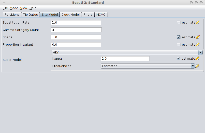
Then, we specify which XML analysis, (we prepared in the previous blog) we want to use to analyse the generated alignment, using

	mergewith = new beast.app.seqgen.MergeDataWith(template="analysis.xml", output="analysis-out.xml");

Now, we have all the components ready to set up the sequence simulator:

	sim = new beast.app.seqgen.SequenceSimulator(data=data, tree=tree, sequencelength=10000, outputFileName="gammaShapeSequence.xml", siteModel=sitemodel, branchRateModel=clockmodel, merge=mergewith);
	sim.run();

This produces gammaShapeSequence.xml and merge it with analysis.xml to get analysis-out.xml. Now we can run the analysis using:

	mcmc = (new XMLParser()).parseFile(new File("analysis-out.xml"));
	mcmc.run();

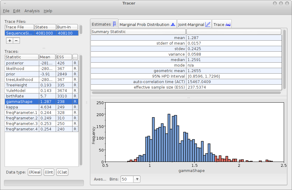
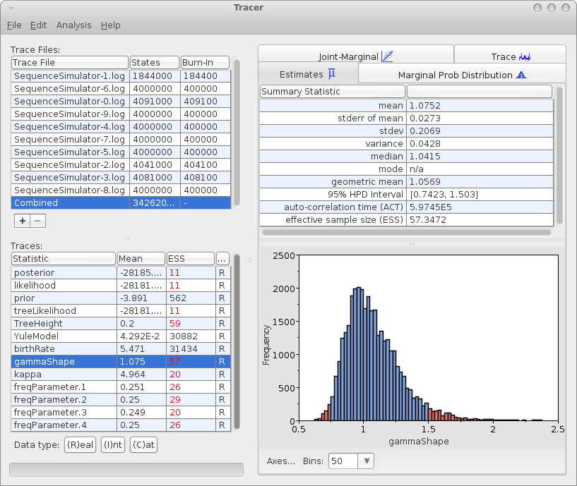
After this finished in a minute or so, we grab estimates from the analysis using the LogAnalyser, and store it in the estimate list.

	log = new LogAnalyser(new String[]{"SequenceSimulator.log"}, 2000, 10);
	s = log.getMean("gammaShape");
	estimate.add(s);

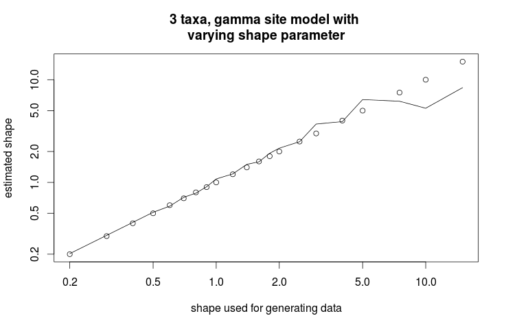
After we have done this for all generated shape parameter values, we can draw a scatter plot and save to “Sample_Chart.png”, using

p = new Plot(x=shapes, y=estimate, title="Gamma shapensimulation", xAxisTitle="original", yAxisTitle="estimate", chartType="Scatter", isYAxisLogarithmic=true, isXAxisLogarithmic=true, output="png");

This analysis just overwrites log files for each generated alignment. To tell BEAST to overwrite, we need

Logger.FILE_MODE = beast.core.Logger.LogFileMode.overwrite;

Furthermore, we want to use BEAGLE, but dependeing on your hardware, this may not speed things up. Setting BEAGLE flags can be done like so:

beagleFlags = beagle.BeagleFlag.VECTOR_SSE.getMask() | beagle.BeagleFlag.PROCESSOR_CPU.getMask();
System.setProperty("beagle.preferred.flags", Long.toString(beagleFlags));

Running the analysis

So, that gives us the following complete script.

// This script demonstrates a simulation study for the
// shape parameter in the gamma rate heterogeneity model.
// Requirements: the file analysis.xml must be in the directory
// from where this script is run.

import beast.evolution.substitutionmodel.*;
import beast.evolution.sitemodel.*;
import beast.evolution.alignment.*;
import beast.util.*;
import beast.core.*;
import com.xeiam.xchart.*;
import beast.app.shell.*;

Logger.FILE_MODE = beast.core.Logger.LogFileMode.overwrite;

// set up flags for BEAGLE -- YMMV
beagleFlags = beagle.BeagleFlag.VECTOR_SSE.getMask() | beagle.BeagleFlag.PROCESSOR_CPU.getMask();
System.setProperty("beagle.preferred.flags", Long.toString(beagleFlags));

// draw gamma shape from the prior (exp(1.0))
shapes = rexp(100, 1.0);
estimate = new ArrayList();

// set up model to draw samples from
data = new Alignment(
		sequence=new Sequence(taxon="human",value="?"),
		sequence=new Sequence(taxon="bonobo",value="?"),
		sequence=new Sequence(taxon="chimp",value="?")
	);
tree = new beast.util.TreeParser(newick="(human:0.2,(chimp:0.15,bonobo:0.15):0.05)", taxa=data, IsLabelledNewick=true);
hky = new HKY(kappa="5.0", frequencies=new Frequencies(data=data));
clockmodel = new beast.evolution.branchratemodel.StrictClockModel("1.0");

k = 0;
for (shape0 : shapes) {
	sitemodel = new SiteModel(gammaCategoryCount=4, substModel=hky, shape=""+shape0);
	//sim = new beast.app.seqgen.SequenceSimulator(data=data, tree=tree, sequencelength=10000, outputFileName="gammaShapeSequence.xml", siteModel=sitemodel, branchRateModel=clockmodel);
	// produce gammaShapeSequence.xml
	//sim.run();
	
	mergewith = new beast.app.seqgen.MergeDataWith(template="analysis.xml", output="analysis-out.xml");
	sim = new beast.app.seqgen.SequenceSimulator(data=data, tree=tree, sequencelength=10000, outputFileName="gammaShapeSequence.xml", siteModel=sitemodel, branchRateModel=clockmodel, merge=mergewith);
	// produce gammaShapeSequence.xml and merge with analysis.xml to get analysis-out.xml
	sim.run();

	// run the analysis
	mcmc = (new XMLParser()).parseFile(new File("analysis-out.xml"));
	mcmc.run();

	// grab estimate from the analysis
	log = new LogAnalyser(new String[]{"SequenceSimulator.log"}, 2000, 10);
	s = log.getMean("gammaShape");
	print("iteration: " + (k++) + " shape = " + shape0 + " estimate = " + s);
	estimate.add(s);
}

// create scatter plot and save to /tmp/Sample_Chart.png
p = new Plot(x=shapes, y=estimate, title="Gamma shapensimulation", xAxisTitle="original", yAxisTitle="estimate", chartType="Scatter", isYAxisLogarithmic=true, isXAxisLogarithmic=true, output="png");

You can run the analysis in BEASTStudio, but you can also run it from the command line, which is probably a bit faster. BEASTShell has a command line interpreter that can be started with

java -cp beast.jar:bsh.jar bsh.Interpreter examples/simstudy.bsh

Once you ran the script, something similar to the following image should appear in the file Sample_Chart.png.

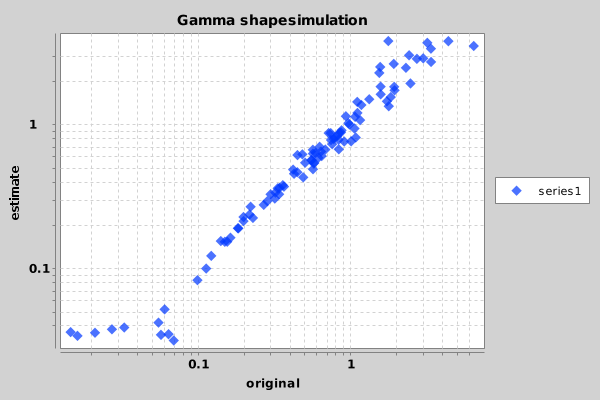
Looks like the shape parameter can be fairly reliably recovered from a large range of shape values. Only at the extremes — below 0.05 and over 15 — the prior is drawing the estimate to the mean.

Simulation studies with BEAST 2

28 April 2014 by Remco Bouckaert

Ever wondered whether the gamma shape that is estimated has any relation to the gamma shape that generated the data? Probably not, but there are many cases where you want to find out whether a model that you use has any relation to the process that generated the data. If so, you probably want to do a simulation study and observe how parameters that generate sequence data have an impact on the parameters of the model that you use to analyse the data.

BEAST has a number of tools that you can use to do a simulation study. Here, we will check what will happen when you change the rate heterogeneity and how it impacts the gamma shape estimate when using the gamma rate heterogeneity model.

Generating an alignment

First of all, we will set up a simulator using the SequenceSimulator class in BEAST. At the time of writing, no GUI is available, so some XML hacking is required.

We will generate a sequence from a 3 taxa fixed tree using the HKY substitution model (kappa=5) and 4 rate categories with gamma shape ranging from 0.2 to 15. The following XML shows how to do this:


        ?
        ?
        ?


			1.0


If you save the XML as simluator.xml you can run it using BEAST, and it will produce a file called gammaShapeSequence.xml containing a sequence alignment with 10000 characters.

Setting up an analysis

Next step is to create a BEAST MCMC analysis file. The easiest way to do this is using BEAUti. Open BEAUti using the (default) Standard template. Import the alignment from the generated file gammaShapeSequence.xml. Go to the Sitemodel panel, and change the substitution model to HKY. Then, set the number of categories to 4, and click the estimate checkbox next to the shape. The panel should look something like this:

Save the file as analysis.xml. After running the analysis with BEAST, and using tracer to inspect the log file SequenceSimulator.log, tracer could report something like this:

As you can see, the gamma shape is estimated as 1.287 with a 95% HPD Interval of [0.8596, 1.7296], so the original gamma shape value of 1.0 is in the 95% HPD Interval. So, it appears that the gamma shape parameter can be estimated. How about the bias? Perhaps we should run the simulation a few more time and see how it behaves over say 10 independently generated alignments.

Repeating this 10x

To repeat the above — simulate sequences, merge with an analysis, and run the analysis — say 10 times, we can adjust the XML script simply by adding the following:

  • Add an iterations attribute to the run element, setting iterations="10".
  • Add a merge element indicating that the generated alignment should be merged with the XML representing an analysis — it replaces the alignment in a BEAST XML file with the one generated by the SequenceSimulator. Since we just created the file analysis.xml with the kind of analysis we want to run, we can use that file.
  • Note that you can specify more than one merge file, and every template file has its alignment replaced with the same generated alignment. This is handy if you want to find out how model misspecification impacts your estimates.

    The XML should look something like this:


            ?
            ?
            ?


    			1.0


    Save as simulator10.xml in the directory containing analysis.xml and when you run the XML file with BEAST, there should be 10 files generated, named analysis-0.xml, analysis-1.xml, up to analysis-9.xml. You could run the ten XML files with BEAST, but you will quickly find out that every log file has the same name — running each file in its own directory, or renaming log files after running an analysis is quite labourious.

    Fortunately The sequence simulator, before it replaces the alignment in the analysis file, replaces every instance of “$(n)” (dollar followed (n)) by the iteration number. So, if we change the file names of the loggers in the analysis.xml file like so:

    From


    to


    And, from


    to


    It is probably also a good idea to set the chainLength="4000000" in analysis.xml. Rerun BEAST on simluator10.xml.

    Now we can run the 10 simulator files and get log file SequenceSimulator-0.log, SequenceSimulator-1.log, … SequenceSimulator-9.log.

    Analysing the log files can be done with tracer with the 10 log files. For the 10 log files, we can select the combined log, which looks something like this:

    The mean estimate over 10 runs is 1.0752 with 95% HPD Interval of [0.7423, 1.503], so the gamma shape used for generating the data is close to the mean and it is firmly in the 95% HPD interval.

    Repeating 10x for 21 different gamma shape values

    So, it looks like the gamma shape value can be infered when the value is 1.0. How about other values? To test this, we can change the simulator.xml file for different values of the shape parameter, and run the analysis 10 times for each gamma shape.

    Analysing with LogAnalyser and R

    Doing this for 21 values of the shape parameter gives 210 log files, which become a bit cumbersome to analyse with tracer. If you would have run the same analysis with a different template (e.g. with a GTR model instead of HKY), you get another 210 log files.

    BEAST has a LogAnalyser that produces similar output to tracer in table format. To run it, you can use

    java -cp beast.jar  beast.util.LogAnalyser trace.log

    Running it on one of the trace logs produces output like this:

    ~> java -cp beast.jar beast.util.LogAnalyser SequenceSimulator-9.log
    Loading SequenceSimulator-9.log skipping 400 log lines
    
    |---------|---------|---------|---------|---------|---------|---------|---------|
    *********************************************************************************
    
    Calculating statistics
    
    |---------|---------|---------|---------|---------|---------|---------|---------|
    ********************************************************************************
    
    item            mean     stderr   stddev   median   95%HPDlo 95%HPDup ACT      ESS      geometric-mean 
    posterior       -28426.3 0.104762 1.962981 -28426.0 -28430.0 -28422.9 10256.42 351.0971 NaN     
    likelihood      -28422.3 0.104126 1.814905 -28422.0 -28425.7 -28419.3 11853.12 303.8017 NaN     
    prior           -4.05647 0.01505  0.768483 -3.79066 -5.60204 -3.26877 1381.170 2607.208 NaN     
    treeLikelihood  -28422.3 0.104126 1.814905 -28422.0 -28425.7 -28419.3 11853.12 303.8017 NaN     
    TreeHeight      0.200092 0.000399 0.006715 0.199813 0.187791 0.213805 12723.26 283.0248 0.19998 
    YuleModel       0.009806 0.013149 0.757205 0.290776 -1.48896 0.721453 1085.933 3316.040 NaN     
    birthRate       5.396959 0.054138 3.102894 4.803029 0.51353  11.32685 1096.214 3284.940 4.521489
    gammaShape      1.198491 0.013759 0.195758 1.186229 0.853668 1.591099 17788.98 202.4286 1.183323
    kappa           4.993622 0.017951 0.231987 4.993078 4.55073  5.396354 21561.68 167.0091 4.988256
    freqParameter.1 0.25509  0.000216 0.003752 0.254981 0.248605 0.262504 11883.76 303.0184 0.255063
    freqParameter.2 0.24809  0.000193 0.003549 0.24805  0.241616 0.255487 10634.58 338.6120 0.248064
    freqParameter.3 0.246065 0.00022  0.003662 0.245816 0.239572 0.25322  13036.39 276.2267 0.246038
    freqParameter.4 0.250755 0.000213 0.003567 0.250743 0.244575 0.258267 12875.19 279.6851 0.250729
    

    For this run, the estimated gamma shape is 1.198491 with an ESS of 202.

    By specifying the prefix directive, you can add a column to identify the run by a prefix value. For example, setting -Dprefix=1.0 like so:

    ~> java -Dprefix=1.0 -cp beast.jar beast.util.LogAnalyser SequenceSimulator-9.log
    
    Loading SequenceSimulator-9.log skipping 400 log lines
    
    |---------|---------|---------|---------|---------|---------|---------|---------|
    *********************************************************************************
    
    Calculating statistics
    
    |---------|---------|---------|---------|---------|---------|---------|---------|
    ********************************************************************************
    
    item            prefix mean     stderr   stddev   median   95%HPDlo 95%HPDup ACT      ESS      geometric-mean 
    posterior       1.0 -28426.3 0.104762 1.962981 -28426.0 -28430.0 -28422.9 10256.42 351.0971 NaN     
    likelihood      1.0 -28422.3 0.104126 1.814905 -28422.0 -28425.7 -28419.3 11853.12 303.8017 NaN     
    prior           1.0 -4.05647 0.01505  0.768483 -3.79066 -5.60204 -3.26877 1381.170 2607.208 NaN     
    treeLikelihood  1.0 -28422.3 0.104126 1.814905 -28422.0 -28425.7 -28419.3 11853.12 303.8017 NaN     
    TreeHeight      1.0 0.200092 0.000399 0.006715 0.199813 0.187791 0.213805 12723.26 283.0248 0.19998 
    YuleModel       1.0 0.009806 0.013149 0.757205 0.290776 -1.48896 0.721453 1085.933 3316.040 NaN     
    birthRate       1.0 5.396959 0.054138 3.102894 4.803029 0.51353  11.32685 1096.214 3284.940 4.521489
    gammaShape      1.0 1.198491 0.013759 0.195758 1.186229 0.853668 1.591099 17788.98 202.4286 1.183323
    kappa           1.0 4.993622 0.017951 0.231987 4.993078 4.55073  5.396354 21561.68 167.0091 4.988256
    freqParameter.1 1.0 0.25509  0.000216 0.003752 0.254981 0.248605 0.262504 11883.76 303.0184 0.255063
    freqParameter.2 1.0 0.24809  0.000193 0.003549 0.24805  0.241616 0.255487 10634.58 338.6120 0.248064
    freqParameter.3 1.0 0.246065 0.00022  0.003662 0.245816 0.239572 0.25322  13036.39 276.2267 0.246038
    freqParameter.4 1.0 0.250755 0.000213 0.003567 0.250743 0.244575 0.258267 12875.19 279.6851 0.250729
    

    This makes it easy to have for example an R script to find the estimates associated with a particular value used for generating the data.

    If you specify more than one indicators, for example the iteration number and the shape parameter, just insert them in braces, like so

    ~> java -Dprefix="1.0 9" -cp beast.jar beast.util.LogAnalyser SequenceSimulator-9.log
    

    The output now has two columns, with headers labeled prefix0 prefix1 and column values 9 1.0

    item            prefix0 prefix1 mean     stderr   stddev   median   95%HPDlo 95%HPDup ACT      ESS      geometric-mean 
    posterior       9 1.0 -28426.3 0.104762 1.962981 -28426.0 -28430.0 -28422.9 10256.42 351.0971 NaN     
    likelihood      9 1.0 -28422.3 0.104126 1.814905 -28422.0 -28425.7 -28419.3 11853.12 303.8017 NaN     
    prior           9 1.0 -4.05647 0.01505  0.768483 -3.79066 -5.60204 -3.26877 1381.170 2607.208 NaN     
    treeLikelihood  9 1.0 -28422.3 0.104126 1.814905 -28422.0 -28425.7 -28419.3 11853.12 303.8017 NaN     
    TreeHeight      9 1.0 0.200092 0.000399 0.006715 0.199813 0.187791 0.213805 12723.26 283.0248 0.19998 
    YuleModel       9 1.0 0.009806 0.013149 0.757205 0.290776 -1.48896 0.721453 1085.933 3316.040 NaN     
    birthRate       9 1.0 5.396959 0.054138 3.102894 4.803029 0.51353  11.32685 1096.214 3284.940 4.521489
    gammaShape      9 1.0 1.198491 0.013759 0.195758 1.186229 0.853668 1.591099 17788.98 202.4286 1.183323
    kappa           9 1.0 4.993622 0.017951 0.231987 4.993078 4.55073  5.396354 21561.68 167.0091 4.988256
    freqParameter.1 9 1.0 0.25509  0.000216 0.003752 0.254981 0.248605 0.262504 11883.76 303.0184 0.255063
    freqParameter.2 9 1.0 0.24809  0.000193 0.003549 0.24805  0.241616 0.255487 10634.58 338.6120 0.248064
    freqParameter.3 9 1.0 0.246065 0.00022  0.003662 0.245816 0.239572 0.25322  13036.39 276.2267 0.246038
    freqParameter.4 9 1.0 0.250755 0.000213 0.003567 0.250743 0.244575 0.258267 12875.19 279.6851 0.250729
    

    Using the LogAnalyser, you can create a text file containing the estimates for all logs. Doing this for various values of gamma shape,

    java -Dprefix=0.2 -cp beast.jar beast.util.LogAnalyser SequenceSimulator-0.2.log >> log.dat
    java -Dprefix=0.3 -cp beast.jar beast.util.LogAnalyser SequenceSimulator-0.3.log >> log.dat
    java -Dprefix=0.4 -cp beast.jar beast.util.LogAnalyser SequenceSimulator-0.4.log >> log.dat
    ...
    java -Dprefix=15.0 -cp beast.jar beast.util.LogAnalyser SequenceSimulator-15.log >> log.dat
    

    You can create a log.dat that you can use in R for a plot. In R, we can do the following — assuming we generated alignments with shape parameter values 0.2, 0.3, 0.4, 0.5, 0.6, 0.7, 0.8, 0.9, 1.0, 1.2, 1.4, 1.6, 1.8, 2.0, 2.5, 3.0, 4.0, 5.0, 7.5,10.0, 15.0:

    > x <- read.table("log.dat",header=1)
    > s <- c(0.2, 0.3, 0.4, 0.5, 0.6, 0.7, 0.8, 0.9, 1.0, 1.2, 1.4, 1.6, 1.8, 2.0, 2.5, 3.0, 4.0, 5.0, 7.5,10.0, 15.0)
    > plot(s,s,log="xy",ann=0);
    > lines(s,as.numeric(as.character(x[which(x$item=="gammaShape"),"mean"])))
    > title("3 taxa, gamma site model with nvarying shape parameter", xlab="shape used for generating data", ylab="estimated shape")
    

    This gives the following graph showing the estimate of shape parameter against the value used for simulating the data. Over all, there is a close match, except for large values of the shape parameter.