Tag Archives: BEAST 2

How much data do I need for SNAPP?

30 June 2015 by Remco Bouckaert

The unwelcome answer to that question is; it depends.

Number of lineages per species

First of all, there should be more than one lineage (= one haploid sequence) for every species. If there is only a single lineage, there are no coalescent events possible in the branches ending in the tips, and the branch above it will have on average only a single coalescent event. This means that the populations sizes for each of the branches will be informed by only a single coalescent event (on average) and there will be very little signal to inform population sizes. The result is that almost certainly, the population size will be sampled from the prior. And since population size and branch lengths are confounded (large population size means larger branch lengths) and the prior on population sizes is quite broad by default, it may take a lot of time to converge.

So, multiple lineages per species is recommended. Of course, this has to be balanced with the penalty in computational that is incurred. So, you have to experiment a bit to find out what is computationally feasible, and how much signal can be obtained from the data.

Sequence length

In SNAPP, every site in a sequence has its own gene tree that is assumed to be independent of all other gene trees. So, adding sites also means adding gene trees.

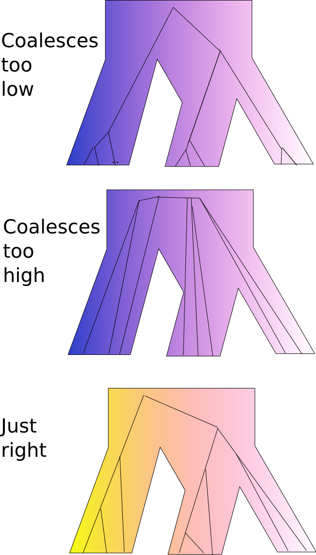
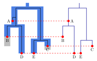
When samples are very closely related, all coalescent events happen very closely to the present time (the sampling time). If so and you look at a branch ending in a species, there is only a single lineage left at the top of the branch. This means we are running in the problem described above; there is no signal in the data left to determine population sizes, and convergence will be difficult. There is no point in adding more sites that have this property, since it would just slow down the calculation without adding more information.

When samples are very distantly related, all coalescent events happen in the branch stemming out of the root. This means, there is no topological information in such samples, and every species tree will fit equally well. On top of this, there is no information to inform population sizes, so SNAPP will not give a lot of information, and will have a terrible time to reach convergence.

In between these extremes, there is the goldilocks zone, where samples coalesc not too early, and not too late, but just in at the right time. In this goldilocks zone, there will be some lineage sorting, so branches above those ending in tips will contain some population size information. This is the kind of data you would like to add.

Of course, it is hard to tell beforehand what kind of data you have, so it is hard to tell beforehand what is the ideal sequence length.


Thanks to David Bryant for pointing out most of the above.

Help, BEAST acts weird! (or how to set up rates)

23 June 2015 by Remco Bouckaert

“What is going wrong?” is an often asked question. There can be many things going wrong, but there is one thing that goes wrong more often than other things and it easy to fix.

The first thing you want to check is the settings of the rates in BEAUti. There are two places where rates are set:

  • The site model panel, where the substitution rate is set
  • The clock model panel where the clock rate is set

The final rate used is the product of these rates.

The way to think of the substitution rate is that it is a relative rate with respect to other partitions, while the clock rate is the overall rate for substitutions per site per year (or any other unit of time you choose to use). So, substitution rates will be numbers close to 1, while clock rates tend to be small numbers, such as 4e-9 substitutions per site per year.

Substitution rates

To set up the substitution rates, use this chart:

Standard analysis

For an analysis using the Standard template, you can go to the clock model tab and use this chart to set up the clock rate:

* Partitions can be ordered arbitrarily. With the first partition I mean the one for which there are either calibrations, tip dates or a rate from the literature, which usually is the first partition listed in the list of clocks, but may be a later one as well.

** Set the clock rate to “1e-x” where x is a number that is somewhere in the region you expect it for your data helps to get through burn-in faster. You could leave it at the default value of 1.0, but it just takes longer to reach convergence. Assuming you are using years as units of time, workable values are 1e-9 for nuclear data, 1e-6 for mitochondrial, bacterial and DNA viral data and 1e-4 for RNA viral data, but if you have more specific information about your sequences it helps to use it to specify starting value.

*BEAST analysis

*BEAST analysis are a bit different in that tip dates are not allowed (at the time of writing) and calibrations are on the species tree, not the gene tree. Usually, all clock rates but the first are estimated using a broad prior. To decide whether the first rate should be estimated or not, use the chart above.

If BEAST still acts weird after rates are set up correctly, just post a question on the BEAST user list.

Better BEAUti templates

16 June 2015 by Remco Bouckaert

When developing a BEAUti template, you have to keep in mind that a BEAST model is directed acyclic graph of BEAST objects such as for example shown here. A BEAUti template describes a sub-graph that can be slotted into the overall model. This means the template has to define two things:

  1. A set of BEAST objects
  2. A set of rules on how to put the sub-network into the full graph

Up to now, the rules on how to connect networks to the graph was through BeautiConnector rules specifying the srcID of one of the BEAST objects in the sub-network, and a targetID and inputName specifying which object in the larger network to connect to. Furthermore, connections are not always necessary; if a parameter is kept fixed instead of estimated, there is no need to log it, so there is no need to connect that parameter to any logger. A BeautiConnector only connects conditional on whatever is specified in the if attribute.

Below is a simple template that specifies the HKY substitution model. The BEAST objects are specified in the CDATA section: the HKY substitution model and its kappa parameter and frequencies object, two operators and a prior on kappa. If kappa is estimated (the default) kappa should be connected to the state (see first connector rule). Likewise for frequencies (second rule).


]]>


Scale HKY transition-transversion
parameter of partition s:$(n)


Exchange values of frequencies of partition s:$(n)


HKY transition-transversion
parameter of partition s:$(n)


From BEAST v2.3.0, the connector rules can be integrated in the XML fragment that specify the BEAST objects. At the top level, the target objects are specified through their IDs, and anything that need to be connected can be inserted through nesting these objects. The conditions are encoded in the if attribute in the beauti namespace, so they look like beauti:if followed by the condition. Let’s walk through the example above.

First, we specify the subtemplate header, and the HKY object:


So far nothing different from above. However, next we will connect the kappa and frequency parameter to the state; just define a state element and specify an idref to the state object. The kappa and frequency parameters will be connected to the stateNode input, for which we specify two stateNode elements, and idrefs to the kappa and frequency parameters specified in the HKY block above.


This replaces the first two connector rules in the original template.

Next, we define the prior on kappa. Since it will be connected to the prior, we wrap it in a distribution element with idref to prior. The condition on which to connect (that kappa is in the likelihood and is estimated) is specified in the prior element. We added name="distribution" in order to ensure the prior is connected to the distribution input.


There is another way to specify conditions which is especially handy when there are several items to be connected that are to be connected under the same condition. The if element specified just inside a top-level element in the CDATA block is interpreted as a condition that applies to all of the elements inside. The condition itself is specified in the cond attribute. For example, the operators can be defined like so;


That leaves the connections to the loggers to be defined;


]]>

And that completes the HKY template.

The hope is that this new way for specifying sub-templates is a bit more intuitive once you are used to writing plain BEAST 2 XML. The idea is that going from an example XML to a sub-template just means

  • remove all XML elements outside sub-graph that is not connected to
  • replace all BEAST objects outside the sub-graph with idrefs
  • add conditions (in beauti:if attributes or if elements)

Then the only thing left is to rename IDs so they math partition information and wrap the BEAUti subtemplate bits around the CDATA section.

Sampling tip dates

9 June 2015 by Remco Bouckaert

To sample the height of leaf nodes, you need to do the following:

  1. Set up a calibration on the tip you want to sample.
  2. Add an operator for scaling the tip.
  3. Add an entry to the logger if you want to log the leaf height

Tip calibration in BEAUti

To set up a calibration, the easiest way to do this is by adding a calibration in BEAUti: in the priors panel, hit the little plus (‘+’) button at the bottom of the screen, then specify the leaf you want to sample and give it a unique name. After hitting the OK button, open the details of the prior by pressing the little triangle next to the taxonset (here Homo_sapiens.prior) and a screen shows up like this:

Make sure the Tipsonly box is checked. If you have multiple tips with the same calibration you can put all of these in the same taxonset. With the tipsonly-flag set, the calibration will be applied to the leafs instead of the most recent common ancestor of the set of tips.

Tip calibration in XML

You can also use add an MRCAPrior to the XML inside the distribution element with id=”prior” like so:


Make sure taxon id’s are unique: it is possible a taxon with the id of the tip you want to sample is already specified elsewhere in the XML. If so, when starting BEAST, you will get an error saying something like

Error 104 parsing the xml input file

IDs should be unique. Duplicate id 'Homo_sapiens' found

identifying the id that was already specified.

Also, you want to point to the right tree specified by tree="@Tree.t:tree" in the fragement above.

Tip sample operator in XML

Once the calibration is set up, for each tip you want to sample add an operator to the XML like so:


and edit it as follows:

  • Make sure the id is unique, just changhing the number will do that.
  • The taxonset attribute should refer to the correct taonset.
  • Check that the tree attribute points to the tree you want to sample from. It should be the same tree as in the MRCAPrior.

Add logger entry

To log the leaf height in the trace log, so you can see its mean height, as well as check how well it mixes, add an entry referring to the MRCAPrior to the tracelog. Just place a log entry inside the logger with id=”tracelog” like so:


That’s all.

Species Delimitation with BEAST

2 June 2015 by Remco Bouckaert

A few weeks back I attended the conference on Species delimitation in the age of genomics at ANU, which made me realise there is quite an interest in the topic. So, here a quick review of methods for species delimitation available in BEAST. The main methods are

  • Bayes factor delimitation (BFD)
  • Threshold based methods DISSECT/STACEY

Bayes factor delimitation

BFD is based on the multi-species coalescent where there two or more scenarios for species assignments. These scenarios can differ in that taxa for different species can be merged, split or you can even test whether a lineage fits better with one species than another.

The multi-species coalescent can be based on *BEAST or SNAPP, depending on the kind of data that you have: gene sequences for *BEAST and SNP or AFLP data for SNAPP. The idea of BFD is based on a fundamental method of Bayesian methods, which is comparing models based on their marginal likelihoods. Note that this is different from the likelihood typically shown in Tracer; the marginal likelihood is the likelihood marginalised over all parameters in the model.

              prior x likelihood
posterior =  --------------------
              marginal likelihood

The marginal likelihood is most reliably calculated using a stepping stone analysis, though this can be quite tedious to estimate since it is rather computational intensive. There are other methods for model fit, like AICM, that are less computational intensive, but these tend to be less reliable (as outlined by Ayden et al, PloS one, 2014).

For each of the scenarios, you set up a *BEAST or SNAPP analysis with a different species assignment, and estimate the marginal likelihood for each of these scenarios. To do this in BEAST, you need the MODEL_SELECTION package. There are more details here on how to set up a stepping stone/path sampling analysis.

Once you have the marginal likelihoods for each of your scenarios, the Bayes factor comparing say scenario A and B is just the difference between the marginal likelihood estimates.

Threshold based methods DISSECT/STACEY

Threshold based methods are based on setting a level epsilon and declare any split in the species tree that is below that value to be within a species, while any split above the threshold is deemed to represent the birth of a new species. The benefit of this method is that it can be performed during an MCMC run, so it does not require a stepping stone analysis. Also, it does not require setting up different scenarios. However, it does require setting a rather arbitrary threshold, though at the meeting at the ANU conference it was argued by various speakers that defining species is to some extent a social construct, which involves some subjective criteria. So, perhaps this is not such a big deal. update: Graham Jones clarified that the threshold is an approximation to zero without any biological meaning, so should not be interpreted as a social construct but its choice is based on a balance of accuracy and speed.

The DISSECT and STACEY packages allows you to do threshold based species delimitation. STACEY is *BEAST on steroids, with DISSECT as species delimitation method. It integrates out population sizes for the branches, which helps convergence though it means that population size information is lost. Furthermore, it has a number of MCMC proposals that help in mixing; a *BEAST analysis can easily get stuck in an area of tree space that forms a local optimum where the species tree gets locked into a topology because one or more of the gene trees have a good fit to the data preventing the species tree to move to alternative topologies. STACEY offers three extra proposals on top of the standard *BEAST proposals that help to get out of these local optima.

A STACEY analysis can be set up in BEAUti, but DISSECT requires a bit more handwork in editing the XML. For STACEY, you need to select the STACEY template under the File/Templates menu to get started. Both need a bit of fiddling with the XML to get going — see documentation for these packages to work out the details.

After running a DISSECT or STACEY XML file through BEAST, you can use the SpeciesDelimitationAnalyser to process the log files and find out the distribution over species assignments.

Threshold methods have been tested for *BEAST, though should work without too much hassle with SNAPP. The prior for SNAPP needs to be replaced with the

Links

BFD paper for *BEAST.

BFD* paper for SNAPP.

Tutorial for BFD*, with example data.

DISSECT paper, also at bioRxiv.

STACEY info and preprint.

Sampled Ancestor Trees in BEAST

1 September 2014 by Remco Bouckaert

Sampled ancestor trees are trees where the nodes that are sampled need not necessarily be leaf nodes, but can be internal nodes of degree two — that is, they only have one parent (as per usual) and one child. This is useful in the case where there are fossils that represent direct ancestors ofa number of extant species. Another situation is where there is epidemiological data and a patient is sampled multiple times, or an individual was sampled and caused infections which were sampled later. Then earlier samples will be ancestors of later samples. To use sampled ancestors trees in BEAST, you need the sampled ancestor package (easiest to install in BEAUti using the File/Manage Packages menu).

Why use sampled ancestor trees instead of binary trees?

In a transmission tree — trees representing an epidemic — some samples will most likely be direct ancestors of later samples. To ensure correct estimation of parameters, like birth rate or substitution rate, models with sampled ancestors should be used for data where direct ancestors are likely to be present. Not accounting for sampled ancestors leads to biases in parameter estimates. For example, the birth rate lambda will be overestimated if you run with binary trees since there are more birth events in a binary tree than in a sampled ancestor tree. Furthermore, if you want to know who exactly infected who, this is not quite as clear in a binary tree as in a sampled ancestor tree.

Likewise, when you model fossil as part of the speciation process (that is, fossils are samples from the process) then considering binary trees in stead of sampled ancestor trees will introduce biases in estimates of divergence times. The tree prior models the fossilisation process, and parameters in the prior will have a bias in their estimate if binary trees are used.

Tree priors for sampled ancestor trees

The SABDSamplingThroughTimeModel is the default sampled ancestor birth-death-sampling tree prior in the sampled ancestors package. It has the following parameters:

  • lamba: birth rate
  • mu: removal rate
  • psi: sampling rate
  • r: probability an individual is removed after sampling.
  • rho: probability of sampling extant species/contemporary individuals.

For the fossilisation process, r=0 because any sample will never be removed, so any of its descendants can be sampled. For r=1, there never is a sampled ancestor. In epidemics r=1 indicates the individuals is removed from the edidemic by sampling. For the transmission process in an epidemic, r is close to 1, depending on type of infection — e.g. it was found to be 0.8 for HIV.

rho is used for contemporary sampling only. It represents the proportion of samples taken out of complete population. For fossilisation, typically rho is close to 1, that is, almost all species relevant to the analysis (belonging to the clade) will be sampled. For epidemics, samples are not contemporary but serially sampled, so rho is not specified.

There is parameter unidentifiability (see this paper) when rho=0.

The birth death sampling model can be used in combination with the skyline model (implemented in the SABDSkylineModel class) where the time spanned by the tree is divided into a number of intervals. Each of these intervals can have its own lambda, mu, psi, r, rho, but they can be shared among intervals as well. For example, you can have a constant mu and psi throughout time, but a different lambda for each interval.

The number of intervals for the skyline model depends on number of times that rates can be expected to be shifted. For instance, if no samples were taken before 1980, but samples are available after 1980, there is a rate shift in sampling rate (psi), so t=1980 is a boundary, and you can specify only psi changed, but that lambda, mu, r (and rho=0) remain the same through the two intervals.

Typically, no sequence data is available for fossils. Without sequence data on fossils, there is no information to infer the tree. In this case, in order to be able to infer the tree, you need at least one parameter, e.g. a strong prior on rho, and lambda, mu and psi can be estimated (r=0). Without fixing rho, all fossils will probably become sampled ancestors, and time estimates will become biased and be estimated too low.

Setting up an analysis

Assuming you set up an analysis in BEAUti say with a Yule model, first of all the tree needs to be replaced by a sampled ancestor tree, the tree operators need to be replaced by those for sampled ancestor trees, so the tree can jump between nodes being ancestors and those being leafs. Further, the Yule model needs to be replaced by the appropriate tree prior, either SABDSamplingThroughTimeModel or SABDSkylineModel.

See the examples in the example directory of the sampled ancestor package for more details.

Load Balancing

18 August 2014 by Remco Bouckaert

If you have a good graphics cards, you can use it with BEAGLE to increase the speed of BEAST runs. If you have multiple graphics cards, when starting BEAST from the command line, the -beagle_order flag can be used to tell which thread goes on which GPU. Start BEAST with the -beagle_info flag to find out what kind of hardware you have and which numbers they are.

For example, I get on my aging univesity computer, the following output:

                  BEAST v2.2.0 Prerelease, 2002-2014
       Bayesian Evolutionary Analysis Sampling Trees
                 Designed and developed by
Remco Bouckaert, Alexei J. Drummond, Andrew Rambaut and Marc A. Suchard
                              
               Department of Computer Science
                   University of Auckland
                  remco@cs.auckland.ac.nz
                  alexei@cs.auckland.ac.nz
                              
             Institute of Evolutionary Biology
                  University of Edinburgh
                     a.rambaut@ed.ac.uk
                              
              David Geffen School of Medicine
           University of California, Los Angeles
                     msuchard@ucla.edu
                              
                Downloads, Help & Resources:
              	http://beast2.cs.auckland.ac.nz
                              
Source code distributed under the GNU Lesser General Public License:
              	http://code.google.com/p/beast2
                              
                     BEAST developers:
	Alex Alekseyenko, Trevor Bedford, Erik Bloomquist, Joseph Heled, 
	Sebastian Hoehna, Denise Kuehnert, Philippe Lemey, Wai Lok Sibon Li, 
	Gerton Lunter, Sidney Markowitz, Vladimir Minin, Michael Defoin Platel, 
          	Oliver Pybus, Chieh-Hsi Wu, Walter Xie
                              
                         Thanks to:
    	Roald Forsberg, Beth Shapiro and Korbinian Strimmer

BEAGLE resources available:
0 : CPU
    Flags: PRECISION_SINGLE PRECISION_DOUBLE COMPUTATION_SYNCH EIGEN_REAL EIGEN_COMPLEX SCALING_MANUAL SCALING_AUTO SCALING_ALWAYS SCALING_DYNAMIC SCALERS_RAW SCALERS_LOG VECTOR_SSE VECTOR_NONE THREADING_NONE PROCESSOR_CPU


1 : GeForce GTX 295
    Global memory (MB): 896
    Clock speed (Ghz): 1.24
    Number of cores: 240
    Flags: PRECISION_SINGLE PRECISION_DOUBLE COMPUTATION_SYNCH EIGEN_REAL EIGEN_COMPLEX SCALING_MANUAL SCALING_AUTO SCALING_ALWAYS SCALING_DYNAMIC SCALERS_RAW SCALERS_LOG VECTOR_NONE THREADING_NONE PROCESSOR_GPU FRAMEWORK_CUDA


2 : GeForce GTX 295
    Global memory (MB): 895
    Clock speed (Ghz): 1.24
    Number of cores: 240
    Flags: PRECISION_SINGLE PRECISION_DOUBLE COMPUTATION_SYNCH EIGEN_REAL EIGEN_COMPLEX SCALING_MANUAL SCALING_AUTO SCALING_ALWAYS SCALING_DYNAMIC SCALERS_RAW SCALERS_LOG VECTOR_NONE THREADING_NONE PROCESSOR_GPU FRAMEWORK_CUDA


3 : GeForce GTX 295
    Global memory (MB): 896
    Clock speed (Ghz): 1.24
    Number of cores: 240
    Flags: PRECISION_SINGLE PRECISION_DOUBLE COMPUTATION_SYNCH EIGEN_REAL EIGEN_COMPLEX SCALING_MANUAL SCALING_AUTO SCALING_ALWAYS SCALING_DYNAMIC SCALERS_RAW SCALERS_LOG VECTOR_NONE THREADING_NONE PROCESSOR_GPU FRAMEWORK_CUDA


4 : GeForce GTX 295
    Global memory (MB): 896
    Clock speed (Ghz): 1.24
    Number of cores: 240
    Flags: PRECISION_SINGLE PRECISION_DOUBLE COMPUTATION_SYNCH EIGEN_REAL EIGEN_COMPLEX SCALING_MANUAL SCALING_AUTO SCALING_ALWAYS SCALING_DYNAMIC SCALERS_RAW SCALERS_LOG VECTOR_NONE THREADING_NONE PROCESSOR_GPU FRAMEWORK_CUDA

It shows there are 4 GPUs numbered 1 to 4 as well as a CPU numbered 0. It also reports some statistics like the number of cores and memory on each GPU. I understand that on OSX due to a bug in the OpenCL library the reported statistics are somewhat exaggerated (e.g. it reports 280 cores on my Macbook air while the HD Graphics 5000 only has 40).

If I have an analysis with two partitions, or one partition, but using the ThreadedTreeLikelihood instead of the TreeLikelihood, and I would start a job with

beast -beagle_order 2,4 -threads 2 beast.xml

it will use two threads, and the first will use GPU number 2 and the second will use GPU number 4. So, you can divide your data among these cards such that all of your GPUs are utilised.

But what if your dataset is too large to fit on one or more of your GPUs? Then, using the -beagle_order flag can be used with some of the partitions using GPUs and others using CPUs. Say, you have a single GPU numbered 1, and a CPU numbered 0, then using

beast -beagle_order 0,0,0,1 -threads 4 beast.xml

will place the first three threads on the CPU and the last on the GPU. Typically, the CPU and GPU do not run at the same speed and I’ll assume the GPU is much faster. What you will see when running the above is then that the three CPU threads are running behind the GPU. So, the GPU thread will be waiting on the CPU threads to finish, and this shows up in CPU load being well below 400% On Mac or Linux I use ‘top’ to see how much CPU load there is. If you could put less data on the CPUs and more on the GPU, you could utilise your computer more efficient.

Now you can — this requires BEAST v2.2.0-pre release, and BEASTlabs for v2.2.0. The ThreadedTreeLikelihood has a proportions attribute where you can specify how much of the data should go into a thread. By default, the ThreadedTreeLikelihood splits up the data in equal parts, which is fine if you only use CPU or only GPU. But when you mix, the proportions specifies proportions of patterns used per thread as space delimited string. This is useful when using a mixture of BEAGLE devices that run at different speeds, e.g GPU and CPU. The string is duplicated if there are more threads than proportions specified. For example, ‘1 2′ as well as ’33 66’ with 2 threads specifies that the first thread gets one third of the patterns and the second two thirds. With 3 threads, it is interpreted as ‘1 2 1’ = 25%, 50%, 25% and with 7 threads it is ‘1 2 1 2 1 2 1’ = 10% 20% 10% 20% 10% 20% 10%. If not specified, all threads get the same proportion of patterns.

By keeping an eye on CPU utilisation, you can see how changing proportions have an impact on CPU load.

Note that mixing the -beagle_GPU and -beagle_SSE flag causes all threads to use CPUs, so the CPU necessarily cannot use the SSE instructions, which means in most practical cases some speed is lost.

The coalescent SIR model in BEAST

18 August 2014 by Remco Bouckaert

Today, we have a look at Volz’s coalescent SIR model, which is an epidemic model that assumes there are three states: susceptible (S), infected (I) and removed (R). To use it, you need to install the phylodynamics package through the package manager. You might want to use coalescent SIR instead of birth-death SIR (BDSIR) — also in the phylodynamics package — since the coalescent model can give smaller confidence intervals.

The coalescent SIR model

The model allows you to estimate the basic reproduction number, R0, which is the average number of people that become infected by each one that is infected. R0 is important, since it mostly determines the size of an epidemic. Other parameters in the model are the transmission rate beta, which is the rate at which new infections arise and the removal rate, gamma. Gamma is often called ‘recovered’ instead of ‘removed’, but since there are other ways to get into state R (by patients dying, or by becoming a sample in our data) the term ‘removed’ is more accurate. Beta and Gamma can be interpreted as birth and death rates, moving from susceptible state S into the infected state I and from the infected state I into removed state R. Further, there is the initial size of susceptible population S0 and time of origin of the infection z0. Obviously, z0 must always be before the root of the tree. At z0, it is assumed there is just a single infected person and throughout the epidemic the population size is constant at size S0+1. For more information, see this paper.

In summary, we have

  • R0, basic reproduction number
  • beta, transmission rate
  • gamma, removal rate
  • S0, initial number of susceptibles
  • z0, time of origin.

Some of these parameters are functionally related through R0=beta*S0/gamma. This means, you can estimate either R0 or beta, and all the others, and then calculate R0 or beta through the formula. There are two implementations: a deterministic and a stochastic one. The stochastic model simulates trajectories of S, I, and R by a jump process while the deterministic model solve a set of ODEs for S, I and R. The stochastic model is much slower — it can be 3 times slower than deterministic — however, stochastic processes more closely represent reality and incorporating them may significantly affect the inference in some cases. For large R0 >1.5 and large S0, deterministic coalescent SIR is both faster and accurate, but for small R0 <1.5 deterministic tends to have the smallest positive bias on R0 and more often have R0 in the 95%HDP (in a simulation study comparing stochastic SIR, deterministic SIR and BDSIR).

Using the model in XML

To use the model, you incorporate serially sampled data by specifying a date trait for sequences.

First, add state nodes to the state element — values need to be adapted for your analysis. Good values help in getting convergence — bad values may result in the chain getting stuck. Makes sure the origin is old enough that it comes before the root of the tree. An error will be thrown when it does not. Here, we estimate R0, and derive beta, so there is no state node for beta.

To set S0 take an estimate of the population size of the area susceptible to the epidemy.
Basic reproductive number R0 must be larger than 1 (otherwise there will be no epidemic) and people disagree on what a high value of R0 is — some say 2.5, but others think 10 is possible.
Gamma removal rate: a high gamma (like in the current ebola outbreak) means fewer overall infected people, high chance of death or quarantine, or recovery with immunity.
z0 must be above root of initial tree, but setting it too high means burn-in may take a long time, so lower values are recommended.


Add priors to element with id=”prior” for S0, R0, gamma and origin — these are just default priors, but if you have more information you should adapt these. For origin z0 – typically not much info available, so uniform with a limited upper bound will do. Note uniform[0,100] means there is 99% that origin is over 1 — check your units of time whether this is relevant for your analysis.


The CSIR model is effectively a tree prior, so we add it to the element with id=”prior”. This adds a deterministic CSIR prior to the analysis (for stochastic CSIR, see below):


Now, we add operators — in this case beta is solved through R0=beta*S0/gamma, so only operators for S0, gamma, R0 and origin are added:


If you have an up-down operator for clock and tree, add origin


If you want to know what the parameters are, add loggers to the trace-log:


Run the analysis in BEAST. There are R scripts (ask Alex Popinga) to get nice plots from these.

The stochastic coalescent SIR model

To add the stochastic CSIR model instead of the deterministic one, the only difference is that the tree prior should be replaced by this:


It is best to set minTraj=1 and minTrajSuccess=1 initially. If there are mixing problems, increase minTraj and minTrajSuccess (minTrajSucces<=minTraj). Increasing numSamplesFromTrajectory will slow things down considerably. 101 tends to be good enough, but in bad mixing increasing it may help, but will slow things down more than increasing minTraj, so try that first.

Coming up

There should be a BEAUti template soon so you can select Coalescent SIR as tree prior and do not worry about the details of the XML.

BEAST Apps for the AppStore

4 August 2014 by Remco Bouckaert

Say, you have some post-processing classes written for your package and you want to make it available to users. Since the class is in your package, say mypackage.addon.jar and most likely you need classes from BEAST-core or other packages, it is a nuisance to set the class path from the command line. You’ll and up having to do something like

java -cp /path/to/beast/lib/beast.jar:~/.beast/2.1/MyPackage/lib/mypackage.addon.jar beast.app.tools.MyTool arg1 arg2 arg3

This is especially cumbersome to explain to users since these paths depend on where BEAST is installed and where packages are installed. These paths are operating system dependent. One solution to this is to use the BEAST AppStore. This is an application that comes with BEAST. It picks up information from the version.xml file. You specify an addonapp element with a description, class, default arguments and an icon. For example, the model-selection package contains an application to run a path sampling analysis, which is encoded like so:


When you start the AppStore, it will look like this:

If you launch it from the AppStore, you probably want to launch it as a GUI, since Windows and Mac users won’t be able to see any terminal input otherwise. You can write your own GUI in Swing or JavaFX if you like, but there are a few helper classes that make it very easy to write GUI applications with BEAST. The recipe is as follows:

  1. Create a class for your App that derives from beast.core.Runnable.
  2. Specify Inputs for each of the arguments for your application.
  3. Implement the run() method to pick up values from inputs and run your app.
  4. Create a class to launch the App.
  5. Update the version.xml file

Path sample analyser application

Step 1: create class for App

The path sample analyser lives in the class beast.inference.PathSampleAnalyser and derives from beast.core.Runnable.

@Description("Reads logs produces through PathSampler and estimates marginal likelihood")
public class PathSampleAnalyser extends beast.core.Runnable {
}

Step 2: specify inputs

For the path sample analyser, we need a root directory, alpha, number of steps and burnin as a percentage. So, we add the following Inputs to the class.

public Input rootDirInput = new Input("rootdir", "root directory for storing particle states and log files (default /tmp)", "/tmp");
public Input alphaInput = new Input("alpha", "alpha parameter of Beta(alpha,1) distribution used to space out steps, default 0.3" +
		"If alpha <= 0, uniform intervals are used.", 0.3);
public Input stepsInput = new Input("nrOfSteps", "the number of steps to use, default 8", 8);
public Input burnInPercentageInput = new Input("burnInPercentage", "burn-In Percentage used for analysing log files", 50);

Step 3: implement run() method

The actual post-processing happens in the method estimateMarginalLikelihood. The run method just gather info from the inputs and passes it to that worker method.

@Override
public void run() throws Exception {
    // do the work
    double marginalL = estimateMarginalLikelihood(
			stepsInput.get(), 
			alphaInput.get(), 
			rootDirInput.get(), 
			burnInPercentageInput.get());

	// report the result       
	System.out.println("marginal L estimate = " + marginalL);
}

Step 4: Create launcher class

Create a class to launch the App. This is the class that you register in the version.xml file. The following bit of code can be used as a template for your own app — just replace the class for the analyser variable and update name and title. It uses two utility classes beast.app.util.Application and beast.app.util.ConsoleApp (currently in the model-selection package, but it should probably move somewhere else). You can also suppress inputs that you do not want to expose to the user.

package beast.app.tools;

import beast.app.beauti.BeautiConfig;
import beast.app.beauti.BeautiDoc;
import beast.app.draw.BEASTObjectDialog;
import beast.app.draw.BEASTObjectPanel;
import beast.app.util.Application;
import beast.app.util.ConsoleApp;

//command line interface to PathSampleAnalyser
public class PathSampleAnalyser {
		
	public static void main(final String[] args) throws Exception {
		Application main = null;
		try {
			// create the runnable class with application that we want to launch
			beast.inference.PathSampleAnalyser analyser = new beast.inference.PathSampleAnalyser();
			
			// need to set the ID of the BEAST-object
			analyser.setID("PathSampleAnalyser");
			
			// then initialise
			analyser.initAndValidate();
			
			// create BeautiDoc and beauti configuration
			BeautiDoc doc = new BeautiDoc();
			doc.beautiConfig = new BeautiConfig();
			doc.beautiConfig.initAndValidate();

			// This is how you suppress an input that we don't want to expose to the user
			// doc.beautiConfig.suppressPlugins.add(analyser.getClass().getName() + ".input-name");

		
			// create panel with entries for the application
			BEASTObjectPanel panel = new BEASTObjectPanel(analyser, analyser.getClass(), doc);
			
			// wrap panel in a dialog
			BEASTObjectDialog dialog = new BEASTObjectDialog(panel, null);
			if (dialog.showDialog()) {
				dialog.accept(analyser, doc);
				analyser.initAndValidate();

				// create a console to show standard error and standard output
				analyser.consoleApp = new ConsoleApp("PathSampleAnalyser", // name 
						"Path Sample Analyser: " + analyser.rootDirInput.get() // console title
						);

				analyser.run();
			}
		} catch (Exception e) {
			System.out.println(e.getMessage());
			if (main != null) {
				System.out.println(main.getUsage());
			}
		}
	}

}

Update the version.xml file

Add an addonapp element to the version.xml file, so the AppStore can pick it up.


When launching the PathSampleAnalyser from the AppStore, it looks like this:

All about starting trees

28 July 2014 by Remco Bouckaert

Before starting an MCMC run, BEAST uses State Node initialisers to set up the starting trees (and other parameters). Often a good starting tree is already available from another analysis (e.g. a maximum likelihood tree). Though it is against the spirit of MCMC, which guarantees any random starting state will lead to convergence, a good starting tree can help with large analysis to speed up convergence quite a bit. Of course another reason to specify a starting tree is if you want to do an analysis using just a single known tree topology.

We start with standard analysis, but see below for *BEAST analyses.

Standard analysis

For a standard analysis, there are three ways to specify a starting tree

  • a random tree
  • a tree in Newick format
  • a cluster tree, e.g. through UPGMA or neighbour joining

By default, BEAUti uses a RandomTree state-node initialiser to generate a starting tree. If you want to replace it with a Newick tree or cluster tree, first you need to remove (or comment out) the RandomTree element from the XML. For a tree in partition XYZ26, just search for RandomTree and remove the XML fragment with id RandomTree.t:XYZ26. It should look something like this:


        1.0
    

Before removing, make note of the initial attribute (@Tree.t:XYZ26> here) and taxa attribute (@XYZ26 here).

Newick starting tree

After removing the Random tree, in the same place, add a TreeParser using the following fragment


The attributes that you want to specify are

  • id="NewickTree.t:XYZ26" the ID should be unique, so something like NewickTree.t: plus the name of the tree would be suitable.
  • initial="@Tree.t:XYZ26" this refers to the tree being initialised. It should be the same as the initial attribute of the RandomTree that was removed.
  • taxa="@XYZ26" this refers to the alignment and ensures that taxa in the tree are lined with those in the alignment. For BEAST v2.1.x, this must be specified to prevent starting with a mislabelled tree
  • newick="((your,(tree,goes)),here)" obviously needs to be replaced with your own tree in Newick format.

This is all you need to know to set up a starting tree. There are a few optional attributes you can use to make life a bit easier:

  • adjustTipHeights is true by default, which means tips of the tree will be set to zero, or if tip dates are specified to these particular tip dates. By setting to adjustTipHeights="false", tips will be initialised by the heights in the Newick tree.
  • if adjustTipHeights="false" then threshold specifies threshold under which node heights (derived from lengths) are set to zero. This helps when there are numeric issues with adding the lengths.
  • scale scale used to multiply internal node heights during parsing. Useful for importing starting from external programs, for instance, RaxML tree rooted using Path-o-gen.
  • IsLabelledNewick="true" Is the Newick tree labelled (alternatively contains node numbers)?
  • If sLabelledNewick="false" then “offset="1" is the lowest taxa number. The default=1 but 0 is common as well. Taxa numbers are as they are ordered in the alignment referred to with the taxa attribute.

Cluster tree

After removing the Random tree, in the same place, add a ClusterTree with the following fragment


The attributes that you need to specify are id='UPGMATree.t:XYZ26', initial="@Tree.t:XYZ26" and taxa="@XYZ26", which are as for Newick tree (see above).

You can use different clustering algorithms by specifying the clusterType="upgma" attribute.

clusterType Description
single single link
complete complete link
upgma or average UPGMA=average link
mean mean link
centroid centroid
ward Ward’s method
adjcomplete adjusted complete link
neighborjoining neighborjoining
neighborjoining2 neighborjoining2 – corrects tree for tip data, unlike plain neighborjoining

*BEAST analysis

For a *BEAST analysis, the default in BEAUti is to generate a UPGMA tree for the species tree, then generate UPGMA trees for each of the gene trees and fit them inside the species tree. In previous incarnations of BEAST, a random tree was generated for species as well as for gene trees, but gene tree branches ending in leaves were lengthened such that each first coalescence of a gene tree was above the root of the species tree. Though this ensures that the gene trees fit inside the species tree, it leads to long burn-in times.

If you want to use a different starting tree for the species tree, first move (not remove!) the StarBeastStartState element generated by BEAUti to just before the run-element with id="mcmc". BEAUti will have generated some elements inside the start-state (such as the species-tree-prior) that we need elsewhere in the analysis. By moving the init element outside the run element, it will not activate the StarBeastStartState.

The StarBeastStartState looks something like this:


For every gene tree there will be a tree entry in the StarBeastStartState. To replace the species tree with a Newick tree, add the following fragment (at the place where the StarBeastStartState was):


The only thing to set up is the Newick using the newick attribute — all other attributes should be as they are (it is using the species tree, which is identified by the Species partition in every *BEAST analysis generated by BEAUti).

For each of the gene trees, you need to specify a tree as well. You can specify them using a Newick tree as for the Standard analysis (see above). Alternatively, you can use a random tree that is placed ‘above’ the species tree. To do this, you add for the first gene tree (just below the new Species tree start tree):


where you replace the initial='@Tree.t:26' and taxa="@26" attributes to match your tree (instead of 26, as in this example). For every subsequent gene tree, you add (below the first gene start tree):


where you replace the initial='@Tree.t:29' and taxa="@29" attributes to match your tree (instead of 29) and make sure the id is unique.