rates | BEAST2

23 June 2015 by Remco Bouckaert

“What is going wrong?” is an often asked question. There can be many things going wrong, but there is one thing that goes wrong more often than other things and it easy to fix.

The first thing you want to check is the settings of the rates in BEAUti. There are two places where rates are set:

The site model panel, where the substitution rate is set
The clock model panel where the clock rate is set

The final rate used is the product of these rates.

The way to think of the substitution rate is that it is a relative rate with respect to other partitions, while the clock rate is the overall rate for substitutions per site per year (or any other unit of time you choose to use). So, substitution rates will be numbers close to 1, while clock rates tend to be small numbers, such as 4e-9 substitutions per site per year.

Substitution rates

To set up the substitution rates, use this chart:

Standard analysis

For an analysis using the Standard template, you can go to the clock model tab and use this chart to set up the clock rate:

* Partitions can be ordered arbitrarily. With the first partition I mean the one for which there are either calibrations, tip dates or a rate from the literature, which usually is the first partition listed in the list of clocks, but may be a later one as well.

** Set the clock rate to “1e-x” where x is a number that is somewhere in the region you expect it for your data helps to get through burn-in faster. You could leave it at the default value of 1.0, but it just takes longer to reach convergence. Assuming you are using years as units of time, workable values are 1e-9 for nuclear data, 1e-6 for mitochondrial, bacterial and DNA viral data and 1e-4 for RNA viral data, but if you have more specific information about your sequences it helps to use it to specify starting value.

*BEAST analysis

*BEAST analysis are a bit different in that tip dates are not allowed (at the time of writing) and calibrations are on the species tree, not the gene tree. Usually, all clock rates but the first are estimated using a broad prior. To decide whether the first rate should be estimated or not, use the chart above.

If BEAST still acts weird after rates are set up correctly, just post a question on the BEAST user list.

7 July 2014 by Remco Bouckaert

Suppose you have 3 genes and know the rate of one of the genes. How do you set up an analysis in BEAUti?

We call the genes gene1, gene2 and gene3, and the rate is say 2.3 substitutions per site per million year. There are a number of things you can do:

Linked genes

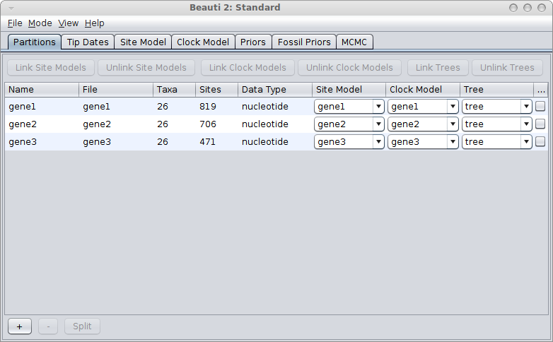
If the genes are linked, for example, because they are all mitochondrial genes, you would use a single tree for all genes. Link trees for all partitions in the partition panel in BEAUti, and it should look something like this:

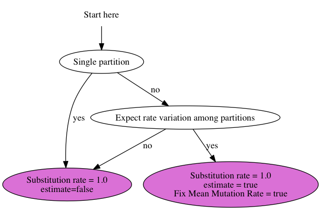
If the rate is known for the first gene, go to the Clock model tab, fill in the clock rate for the gene you have a rate for and BEAUti conveniently fixes the rate for that partition and marks the others as estimated.

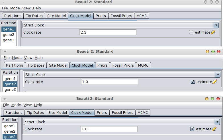
If the gene with the known rate is not the first partition, you have to uncheck the “Mode/Automatic set clock rates”.

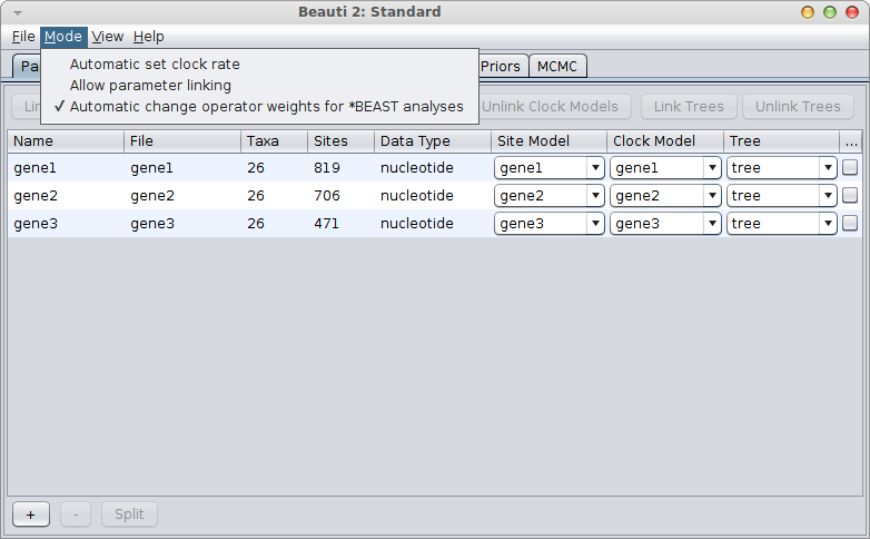
Then go to the clock model panel, where you can set the estimate box for each of the genes you want to estimate and uncheck it for the gene with the known rate.

Independent genes

If all three genes are unlinked, use a *BEAST analysis where you have an independent gene tree for each of your genes. Essentially, the same scenario for clock rates as for the single tree applies.

Semi-independent genes

You can have a mixture of the above scenarios when two genes are linked and one is independent of the two, say, when two genes are mitochondrial and one nuclear. Then, a *BEAST analysis is more appropriate, with two gene trees — one for the linked genes and one for the other.

Uncertainty: rate = 2.3 ± 0.25

Often, there is some measure of uncertainty for the known rate, so instead of 2.3, we find 2.3 ± 0.25 in the literature. Then, it would be more appropriate to estimate the known clock rate as well, and put a strong prior on that clock rate. In this case, you want to uncheck the “Mode/Automatic set clock rates” menu and make sure all clock rates have their “estimate” box ticked in the clock model panel. You set the clock-rate prior in the priors panel.

It is tempting to interpret a rate estimate of 2.3 ± 0.25 as a normal distribution with mean of 2.3 and a 95% confidence interval of [2.3-0.25, 2.3+0.25] = [2.05, 2.55]. However, the problem with a normal distribution is that its range includes negative values. In general, if the mean is more than 4 standard deviations away from zero, this can be reasonable, since less than 0.006% of the probability mass is below zero.

What is wrong with the normal prior?

Even then it is still possible that during the MCMC, the clock rate may become zero (or even negative) and there is no indication from the prior that this is not allowed. This can happen because other priors interact with the rate prior. In particular, the tree priors (e.g. a coalescent when there are enough taxa) can strongly guide the height of the tree, and thus interact with the rate prior. The tree prior should be conditioned on the rate calibration (prior = P(tree|calibration) * P(calibration)), but in BEAST we generally assume (incorrectly) priors are independent (prior = P(tree) * P(calibration)), because we do not know how to do the conditioning. This means, unfortunately, that this interaction is not obvious when sampling from the prior, and when inspecting the trace it seems we are sampling from the normal rate prior that we specified. Only when sampling from the posterior, both priors try to influence the height of the tree, and start interacting with each other.

So, if you insist on using a normal distribution, you must verify that the rate is distributed according to your prior (by inspecting the trace file in Tracer) and the rate does not contain zero or negative values. (You could ensure that the rate remains positive by setting a lower bound on the clock rate).

Use a log-normal prior!

A much better alternative is to use a log-normal prior, which has a range over the positive numbers only. For small values of the standard deviation, it is shaped like a bell-curve. Just like the normal distribution, it only requires two parameters to specify, but requires no lower bound to be set on the rate, since negative values are automatically out of range.

It is easy to configure the log-normal prior in BEAUti, by setting the mean “M” to 2.3, check the “Mean in real space” box (as opposed to in log space) and set the standard deviation “S” by matching the 95% interval to [2.05, 2.55]. This means matching the 2.5% quantile to 2.05 and the 97.5% quantile to approximately 2.55. A bit of fiddling with the numbers shows that S=0.059 is a reasonable match.

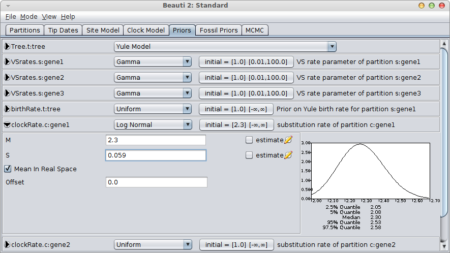
You still want to verify that the rate is distributed according to your rate prior (by inspecting the trace file in Tracer) and is not influenced by the tree prior too much.

BEAST2

Tag Archives: rates

Help, BEAST acts weird! (or how to set up rates)