Category Archives: Blog

Blog

Sampling tip dates

June 9, 2015 rbou019 Leave a comment

9 June 2015 by Remco Bouckaert

To sample the height of leaf nodes, you need to do the following:

Set up a calibration on the tip you want to sample.
Add an operator for scaling the tip.
Add an entry to the logger if you want to log the leaf height

Tip calibration in BEAUti

To set up a calibration, the easiest way to do this is by adding a calibration in BEAUti: in the priors panel, hit the little plus (‘+’) button at the bottom of the screen, then specify the leaf you want to sample and give it a unique name. After hitting the OK button, open the details of the prior by pressing the little triangle next to the taxonset (here Homo_sapiens.prior) and a screen shows up like this:

Make sure the Tipsonly box is checked. If you have multiple tips with the same calibration you can put all of these in the same taxonset. With the tipsonly-flag set, the calibration will be applied to the leafs instead of the most recent common ancestor of the set of tips.

Tip calibration in XML

You can also use add an MRCAPrior to the XML inside the distribution element with id=”prior” like so:

Make sure taxon id’s are unique: it is possible a taxon with the id of the tip you want to sample is already specified elsewhere in the XML. If so, when starting BEAST, you will get an error saying something like

Error 104 parsing the xml input file

IDs should be unique. Duplicate id 'Homo_sapiens' found

identifying the id that was already specified.

Also, you want to point to the right tree specified by tree="@Tree.t:tree" in the fragement above.

Tip sample operator in XML

Once the calibration is set up, for each tip you want to sample add an operator to the XML like so:

and edit it as follows:

Make sure the id is unique, just changhing the number will do that.
The taxonset attribute should refer to the correct taonset.
Check that the tree attribute points to the tree you want to sample from. It should be the same tree as in the MRCAPrior.

Add logger entry

To log the leaf height in the trace log, so you can see its mean height, as well as check how well it mixes, add an entry referring to the MRCAPrior to the tracelog. Just place a log entry inside the logger with id=”tracelog” like so:

That’s all.

Blog

Species Delimitation with BEAST

June 2, 2015 rbou019 Leave a comment

2 June 2015 by Remco Bouckaert

A few weeks back I attended the conference on Species delimitation in the age of genomics at ANU, which made me realise there is quite an interest in the topic. So, here a quick review of methods for species delimitation available in BEAST. The main methods are

Bayes factor delimitation (BFD)
Threshold based methods DISSECT/STACEY

Bayes factor delimitation

BFD is based on the multi-species coalescent where there two or more scenarios for species assignments. These scenarios can differ in that taxa for different species can be merged, split or you can even test whether a lineage fits better with one species than another.

The multi-species coalescent can be based on *BEAST or SNAPP, depending on the kind of data that you have: gene sequences for *BEAST and SNP or AFLP data for SNAPP. The idea of BFD is based on a fundamental method of Bayesian methods, which is comparing models based on their marginal likelihoods. Note that this is different from the likelihood typically shown in Tracer; the marginal likelihood is the likelihood marginalised over all parameters in the model.

              prior x likelihood
posterior =  --------------------
              marginal likelihood

The marginal likelihood is most reliably calculated using a stepping stone analysis, though this can be quite tedious to estimate since it is rather computational intensive. There are other methods for model fit, like AICM, that are less computational intensive, but these tend to be less reliable (as outlined by Ayden et al, PloS one, 2014).

For each of the scenarios, you set up a *BEAST or SNAPP analysis with a different species assignment, and estimate the marginal likelihood for each of these scenarios. To do this in BEAST, you need the MODEL_SELECTION package. There are more details here on how to set up a stepping stone/path sampling analysis.

Once you have the marginal likelihoods for each of your scenarios, the Bayes factor comparing say scenario A and B is just the difference between the marginal likelihood estimates.

Threshold based methods DISSECT/STACEY

Threshold based methods are based on setting a level epsilon and declare any split in the species tree that is below that value to be within a species, while any split above the threshold is deemed to represent the birth of a new species. The benefit of this method is that it can be performed during an MCMC run, so it does not require a stepping stone analysis. Also, it does not require setting up different scenarios. However, it does require setting a rather arbitrary threshold, though at the meeting at the ANU conference it was argued by various speakers that defining species is to some extent a social construct, which involves some subjective criteria. So, perhaps this is not such a big deal. update: Graham Jones clarified that the threshold is an approximation to zero without any biological meaning, so should not be interpreted as a social construct but its choice is based on a balance of accuracy and speed.

The DISSECT and STACEY packages allows you to do threshold based species delimitation. STACEY is *BEAST on steroids, with DISSECT as species delimitation method. It integrates out population sizes for the branches, which helps convergence though it means that population size information is lost. Furthermore, it has a number of MCMC proposals that help in mixing; a *BEAST analysis can easily get stuck in an area of tree space that forms a local optimum where the species tree gets locked into a topology because one or more of the gene trees have a good fit to the data preventing the species tree to move to alternative topologies. STACEY offers three extra proposals on top of the standard *BEAST proposals that help to get out of these local optima.

A STACEY analysis can be set up in BEAUti, but DISSECT requires a bit more handwork in editing the XML. For STACEY, you need to select the STACEY template under the File/Templates menu to get started. Both need a bit of fiddling with the XML to get going — see documentation for these packages to work out the details.

After running a DISSECT or STACEY XML file through BEAST, you can use the SpeciesDelimitationAnalyser to process the log files and find out the distribution over species assignments.

Threshold methods have been tested for *BEAST, though should work without too much hassle with SNAPP. The prior for SNAPP needs to be replaced with the

Links

BFD paper for *BEAST.

BFD* paper for SNAPP.

Tutorial for BFD*, with example data.

DISSECT paper, also at bioRxiv.

STACEY info and preprint.

Blog

What is new in BEAST v2.3.0 and its packages

May 26, 2015 rbou019 Leave a comment

26 May 2015 by Remco Bouckaert

The main improvement is in BEAUti fixes. There are a few bugs, especially with cloning and linking/unlinkig partitions that are fixed. The templates for tree priors have been reorganised, since they some times interferred.

The File-menu in BEAUti is reorganised so it is easier to access files from packages. On the Mac, packages are installed in a rather hard to find folder. With the new menu, it is easy to select a working directory, then import an alignment or open an example file from the package.

The File menu has entries for creating new partitions directly, which saves one click every time an alignment is imported.

The build scripts have been updated so that each applications automatically loads beast.jar instead of having the whole file duplicated in each application, giving smaller footprint for Mac and Windows. This also makes it easier to update using the latest development build; just replace the beast.jar file with the one from here and you are running the development version.

There are a few bug-fixes, in particual, issues with synchronisation affecting ThreadedTreeLikelihood from the BEASTLabs package, a fix in EigenDecomposition affecting asymmetric rate matrices (which caused problems with ancestral reconstruction from the BEAST-CLASSIC package).
Furthre, the code is updated such that dependency on taxon order is reduced, making multiple partition handling more robust

The LogCombiner command line interface is improved so it can take multipe log files as argument, so you can use wildcards to specify multiple files, like so:

logcombiner -log beast.*.log

This version can keep running v2.2 and its packages alongside v2.3, so no need to delete old packages any more.

DensiTree is updated to v2.2.2.

Package added since the last udpate on this blog

There are now 20 packages, many of them added since the last update.

MGSM: multi-gamma site model

Unlike the standard gamma rate heterogeneity model, which uses a single shape parameter, the multi-gamma site model allows the shape parameter to vary over branches. This leads often to better model fit and can result in significantly different divergence time estimates. Preprint on bioRxiv.

Comes with BEAUti support.

Spherial geography

Phyleographical model that assumes heterogeneious diffusion on a sphere, which for large areas can give significantly different results than continuous geography by diffusion on a plane. For a tutorial see here. Preprint on bioRxiv.

Comes with BEAUti support.

bModelTest

A package for nucleotide models that uses reversible jump between a number of substitution models, with and without gamma rate heterogeneity and with and without proportion invariant sites. So, these parts of the model will be estimated during the MCMC run and do not need to be specified beforehand any more. Preprint on bioRxiv.

Comes with BEAUti support.

Morphological-models

Implements the LewisMK model for morphological data, see morphological models. Deals with ambiguities and nexus files for morpholocial data.

Comes with BEAUti support.

Sampled ancestors

Described previously.

The coalescent SIR model

Described previously.

Metroplolis coupled MCMC

Aka MCMCMC or MC3. More here.

Species delimitation with DISSECT and STACEY

Methods for species delimitation based on the multi species coalescent, so this is useful for data that could be analysed using *BEAST. More on this soon.

Bayesian structured coalescent approximation with BASTA

Approximation of the structured coalescent which allows a large number of demes than the pure structured coalescent as for example implemented in the MultiTypeTree package.

Index of 2014 posts

May 19, 2015 rbou019 Leave a comment

Blog

Sampled Ancestor Trees in BEAST

September 2, 2014 rbou019 Leave a comment

1 September 2014 by Remco Bouckaert

Sampled ancestor trees are trees where the nodes that are sampled need not necessarily be leaf nodes, but can be internal nodes of degree two — that is, they only have one parent (as per usual) and one child. This is useful in the case where there are fossils that represent direct ancestors ofa number of extant species. Another situation is where there is epidemiological data and a patient is sampled multiple times, or an individual was sampled and caused infections which were sampled later. Then earlier samples will be ancestors of later samples. To use sampled ancestors trees in BEAST, you need the sampled ancestor package (easiest to install in BEAUti using the File/Manage Packages menu).

Why use sampled ancestor trees instead of binary trees?

In a transmission tree — trees representing an epidemic — some samples will most likely be direct ancestors of later samples. To ensure correct estimation of parameters, like birth rate or substitution rate, models with sampled ancestors should be used for data where direct ancestors are likely to be present. Not accounting for sampled ancestors leads to biases in parameter estimates. For example, the birth rate lambda will be overestimated if you run with binary trees since there are more birth events in a binary tree than in a sampled ancestor tree. Furthermore, if you want to know who exactly infected who, this is not quite as clear in a binary tree as in a sampled ancestor tree.

Likewise, when you model fossil as part of the speciation process (that is, fossils are samples from the process) then considering binary trees in stead of sampled ancestor trees will introduce biases in estimates of divergence times. The tree prior models the fossilisation process, and parameters in the prior will have a bias in their estimate if binary trees are used.

Tree priors for sampled ancestor trees

The SABDSamplingThroughTimeModel is the default sampled ancestor birth-death-sampling tree prior in the sampled ancestors package. It has the following parameters:

lamba: birth rate
mu: removal rate
psi: sampling rate
r: probability an individual is removed after sampling.
rho: probability of sampling extant species/contemporary individuals.

For the fossilisation process, r=0 because any sample will never be removed, so any of its descendants can be sampled. For r=1, there never is a sampled ancestor. In epidemics r=1 indicates the individuals is removed from the edidemic by sampling. For the transmission process in an epidemic, r is close to 1, depending on type of infection — e.g. it was found to be 0.8 for HIV.

rho is used for contemporary sampling only. It represents the proportion of samples taken out of complete population. For fossilisation, typically rho is close to 1, that is, almost all species relevant to the analysis (belonging to the clade) will be sampled. For epidemics, samples are not contemporary but serially sampled, so rho is not specified.

There is parameter unidentifiability (see this paper) when rho=0.

The birth death sampling model can be used in combination with the skyline model (implemented in the SABDSkylineModel class) where the time spanned by the tree is divided into a number of intervals. Each of these intervals can have its own lambda, mu, psi, r, rho, but they can be shared among intervals as well. For example, you can have a constant mu and psi throughout time, but a different lambda for each interval.

The number of intervals for the skyline model depends on number of times that rates can be expected to be shifted. For instance, if no samples were taken before 1980, but samples are available after 1980, there is a rate shift in sampling rate (psi), so t=1980 is a boundary, and you can specify only psi changed, but that lambda, mu, r (and rho=0) remain the same through the two intervals.

Typically, no sequence data is available for fossils. Without sequence data on fossils, there is no information to infer the tree. In this case, in order to be able to infer the tree, you need at least one parameter, e.g. a strong prior on rho, and lambda, mu and psi can be estimated (r=0). Without fixing rho, all fossils will probably become sampled ancestors, and time estimates will become biased and be estimated too low.

Setting up an analysis

Assuming you set up an analysis in BEAUti say with a Yule model, first of all the tree needs to be replaced by a sampled ancestor tree, the tree operators need to be replaced by those for sampled ancestor trees, so the tree can jump between nodes being ancestors and those being leafs. Further, the Yule model needs to be replaced by the appropriate tree prior, either SABDSamplingThroughTimeModel or SABDSkylineModel.

See the examples in the example directory of the sampled ancestor package for more details.

Blog

Load Balancing

August 25, 2014 rbou019 Leave a comment

18 August 2014 by Remco Bouckaert

If you have a good graphics cards, you can use it with BEAGLE to increase the speed of BEAST runs. If you have multiple graphics cards, when starting BEAST from the command line, the -beagle_order flag can be used to tell which thread goes on which GPU. Start BEAST with the -beagle_info flag to find out what kind of hardware you have and which numbers they are.

For example, I get on my aging univesity computer, the following output:

                  BEAST v2.2.0 Prerelease, 2002-2014
       Bayesian Evolutionary Analysis Sampling Trees
                 Designed and developed by
Remco Bouckaert, Alexei J. Drummond, Andrew Rambaut and Marc A. Suchard
                              
               Department of Computer Science
                   University of Auckland
                  remco@cs.auckland.ac.nz
                  alexei@cs.auckland.ac.nz
                              
             Institute of Evolutionary Biology
                  University of Edinburgh
                     a.rambaut@ed.ac.uk
                              
              David Geffen School of Medicine
           University of California, Los Angeles
                     msuchard@ucla.edu
                              
                Downloads, Help & Resources:
              	http://beast2.cs.auckland.ac.nz
                              
Source code distributed under the GNU Lesser General Public License:
              	http://code.google.com/p/beast2
                              
                     BEAST developers:
	Alex Alekseyenko, Trevor Bedford, Erik Bloomquist, Joseph Heled, 
	Sebastian Hoehna, Denise Kuehnert, Philippe Lemey, Wai Lok Sibon Li, 
	Gerton Lunter, Sidney Markowitz, Vladimir Minin, Michael Defoin Platel, 
          	Oliver Pybus, Chieh-Hsi Wu, Walter Xie
                              
                         Thanks to:
    	Roald Forsberg, Beth Shapiro and Korbinian Strimmer

BEAGLE resources available:
0 : CPU
    Flags: PRECISION_SINGLE PRECISION_DOUBLE COMPUTATION_SYNCH EIGEN_REAL EIGEN_COMPLEX SCALING_MANUAL SCALING_AUTO SCALING_ALWAYS SCALING_DYNAMIC SCALERS_RAW SCALERS_LOG VECTOR_SSE VECTOR_NONE THREADING_NONE PROCESSOR_CPU


1 : GeForce GTX 295
    Global memory (MB): 896
    Clock speed (Ghz): 1.24
    Number of cores: 240
    Flags: PRECISION_SINGLE PRECISION_DOUBLE COMPUTATION_SYNCH EIGEN_REAL EIGEN_COMPLEX SCALING_MANUAL SCALING_AUTO SCALING_ALWAYS SCALING_DYNAMIC SCALERS_RAW SCALERS_LOG VECTOR_NONE THREADING_NONE PROCESSOR_GPU FRAMEWORK_CUDA


2 : GeForce GTX 295
    Global memory (MB): 895
    Clock speed (Ghz): 1.24
    Number of cores: 240
    Flags: PRECISION_SINGLE PRECISION_DOUBLE COMPUTATION_SYNCH EIGEN_REAL EIGEN_COMPLEX SCALING_MANUAL SCALING_AUTO SCALING_ALWAYS SCALING_DYNAMIC SCALERS_RAW SCALERS_LOG VECTOR_NONE THREADING_NONE PROCESSOR_GPU FRAMEWORK_CUDA


3 : GeForce GTX 295
    Global memory (MB): 896
    Clock speed (Ghz): 1.24
    Number of cores: 240
    Flags: PRECISION_SINGLE PRECISION_DOUBLE COMPUTATION_SYNCH EIGEN_REAL EIGEN_COMPLEX SCALING_MANUAL SCALING_AUTO SCALING_ALWAYS SCALING_DYNAMIC SCALERS_RAW SCALERS_LOG VECTOR_NONE THREADING_NONE PROCESSOR_GPU FRAMEWORK_CUDA


4 : GeForce GTX 295
    Global memory (MB): 896
    Clock speed (Ghz): 1.24
    Number of cores: 240
    Flags: PRECISION_SINGLE PRECISION_DOUBLE COMPUTATION_SYNCH EIGEN_REAL EIGEN_COMPLEX SCALING_MANUAL SCALING_AUTO SCALING_ALWAYS SCALING_DYNAMIC SCALERS_RAW SCALERS_LOG VECTOR_NONE THREADING_NONE PROCESSOR_GPU FRAMEWORK_CUDA

It shows there are 4 GPUs numbered 1 to 4 as well as a CPU numbered 0. It also reports some statistics like the number of cores and memory on each GPU. I understand that on OSX due to a bug in the OpenCL library the reported statistics are somewhat exaggerated (e.g. it reports 280 cores on my Macbook air while the HD Graphics 5000 only has 40).

If I have an analysis with two partitions, or one partition, but using the ThreadedTreeLikelihood instead of the TreeLikelihood, and I would start a job with

beast -beagle_order 2,4 -threads 2 beast.xml

it will use two threads, and the first will use GPU number 2 and the second will use GPU number 4. So, you can divide your data among these cards such that all of your GPUs are utilised.

But what if your dataset is too large to fit on one or more of your GPUs? Then, using the -beagle_order flag can be used with some of the partitions using GPUs and others using CPUs. Say, you have a single GPU numbered 1, and a CPU numbered 0, then using

beast -beagle_order 0,0,0,1 -threads 4 beast.xml

will place the first three threads on the CPU and the last on the GPU. Typically, the CPU and GPU do not run at the same speed and I’ll assume the GPU is much faster. What you will see when running the above is then that the three CPU threads are running behind the GPU. So, the GPU thread will be waiting on the CPU threads to finish, and this shows up in CPU load being well below 400% On Mac or Linux I use ‘top’ to see how much CPU load there is. If you could put less data on the CPUs and more on the GPU, you could utilise your computer more efficient.

Now you can — this requires BEAST v2.2.0-pre release, and BEASTlabs for v2.2.0. The ThreadedTreeLikelihood has a proportions attribute where you can specify how much of the data should go into a thread. By default, the ThreadedTreeLikelihood splits up the data in equal parts, which is fine if you only use CPU or only GPU. But when you mix, the proportions specifies proportions of patterns used per thread as space delimited string. This is useful when using a mixture of BEAGLE devices that run at different speeds, e.g GPU and CPU. The string is duplicated if there are more threads than proportions specified. For example, ‘1 2′ as well as ’33 66’ with 2 threads specifies that the first thread gets one third of the patterns and the second two thirds. With 3 threads, it is interpreted as ‘1 2 1’ = 25%, 50%, 25% and with 7 threads it is ‘1 2 1 2 1 2 1’ = 10% 20% 10% 20% 10% 20% 10%. If not specified, all threads get the same proportion of patterns.

By keeping an eye on CPU utilisation, you can see how changing proportions have an impact on CPU load.

Note that mixing the -beagle_GPU and -beagle_SSE flag causes all threads to use CPUs, so the CPU necessarily cannot use the SSE instructions, which means in most practical cases some speed is lost.

Blog

The coalescent SIR model in BEAST

August 18, 2014 rbou019 Leave a comment

18 August 2014 by Remco Bouckaert

Today, we have a look at Volz’s coalescent SIR model, which is an epidemic model that assumes there are three states: susceptible (S), infected (I) and removed (R). To use it, you need to install the phylodynamics package through the package manager. You might want to use coalescent SIR instead of birth-death SIR (BDSIR) — also in the phylodynamics package — since the coalescent model can give smaller confidence intervals.

The coalescent SIR model

The model allows you to estimate the basic reproduction number, R0, which is the average number of people that become infected by each one that is infected. R0 is important, since it mostly determines the size of an epidemic. Other parameters in the model are the transmission rate beta, which is the rate at which new infections arise and the removal rate, gamma. Gamma is often called ‘recovered’ instead of ‘removed’, but since there are other ways to get into state R (by patients dying, or by becoming a sample in our data) the term ‘removed’ is more accurate. Beta and Gamma can be interpreted as birth and death rates, moving from susceptible state S into the infected state I and from the infected state I into removed state R. Further, there is the initial size of susceptible population S0 and time of origin of the infection z0. Obviously, z0 must always be before the root of the tree. At z0, it is assumed there is just a single infected person and throughout the epidemic the population size is constant at size S0+1. For more information, see this paper.

In summary, we have

R0, basic reproduction number
beta, transmission rate
gamma, removal rate
S0, initial number of susceptibles
z0, time of origin.

Some of these parameters are functionally related through R0=beta*S0/gamma. This means, you can estimate either R0 or beta, and all the others, and then calculate R0 or beta through the formula. There are two implementations: a deterministic and a stochastic one. The stochastic model simulates trajectories of S, I, and R by a jump process while the deterministic model solve a set of ODEs for S, I and R. The stochastic model is much slower — it can be 3 times slower than deterministic — however, stochastic processes more closely represent reality and incorporating them may significantly affect the inference in some cases. For large R0 >1.5 and large S0, deterministic coalescent SIR is both faster and accurate, but for small R0 <1.5 deterministic tends to have the smallest positive bias on R0 and more often have R0 in the 95%HDP (in a simulation study comparing stochastic SIR, deterministic SIR and BDSIR).

Using the model in XML

To use the model, you incorporate serially sampled data by specifying a date trait for sequences.

First, add state nodes to the state element — values need to be adapted for your analysis. Good values help in getting convergence — bad values may result in the chain getting stuck. Makes sure the origin is old enough that it comes before the root of the tree. An error will be thrown when it does not. Here, we estimate R0, and derive beta, so there is no state node for beta.

To set S0 take an estimate of the population size of the area susceptible to the epidemy.
Basic reproductive number R0 must be larger than 1 (otherwise there will be no epidemic) and people disagree on what a high value of R0 is — some say 2.5, but others think 10 is possible.
Gamma removal rate: a high gamma (like in the current ebola outbreak) means fewer overall infected people, high chance of death or quarantine, or recovery with immunity.
z0 must be above root of initial tree, but setting it too high means burn-in may take a long time, so lower values are recommended.

Add priors to element with id=”prior” for S0, R0, gamma and origin — these are just default priors, but if you have more information you should adapt these. For origin z0 – typically not much info available, so uniform with a limited upper bound will do. Note uniform[0,100] means there is 99% that origin is over 1 — check your units of time whether this is relevant for your analysis.

The CSIR model is effectively a tree prior, so we add it to the element with id=”prior”. This adds a deterministic CSIR prior to the analysis (for stochastic CSIR, see below):

Now, we add operators — in this case beta is solved through R0=beta*S0/gamma, so only operators for S0, gamma, R0 and origin are added:

If you have an up-down operator for clock and tree, add origin

If you want to know what the parameters are, add loggers to the trace-log:

Run the analysis in BEAST. There are R scripts (ask Alex Popinga) to get nice plots from these.

The stochastic coalescent SIR model

To add the stochastic CSIR model instead of the deterministic one, the only difference is that the tree prior should be replaced by this:

It is best to set minTraj=1 and minTrajSuccess=1 initially. If there are mixing problems, increase minTraj and minTrajSuccess (minTrajSucces<=minTraj). Increasing numSamplesFromTrajectory will slow things down considerably. 101 tends to be good enough, but in bad mixing increasing it may help, but will slow things down more than increasing minTraj, so try that first.

Coming up

There should be a BEAUti template soon so you can select Coalescent SIR as tree prior and do not worry about the details of the XML.

Blog

BEAST on OSX trouble shooting

August 11, 2014 rbou019 Leave a comment

11 August 2014 by Remco Bouckaert

Just this week I got a new Mac laptop, and could experience first hand what it is to install BEAST on a virgin machine. There are number of reasons why BEAST will not start on Apple OSX, and we have a look at the most common causes and how to solve them.

DMG is ‘damaged’

First of all, after downloading BEAST and OSX may respond to opening the dmg file by showing a dialog with the message that the file is damaged and offers a choice of deleting or canceling the action.

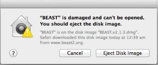
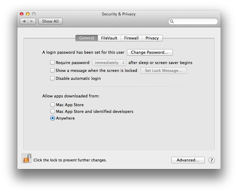
By default, security settings on Mavericks is that only apps downloaded from Mac App Store and from identified developers are opened, and anything else is treated with the message shown above. To fix this, open the security and privacy settings — click the apple icon in the top left corner, then click System Preferences, and select Security & Privacy. A window similar to this will be shown:

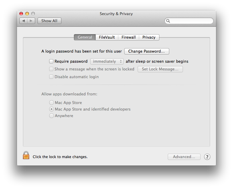
You need to change that to allow apps from anywhere. Once you click that, a window pops up asking whether you want to make your computer less secure. No worries — after starting BEAST once, you can set it back to a more secure setting.

Cannot be opened

Another message that can pop up is that BEAST or BEAUti cannot be opened — something similar to this

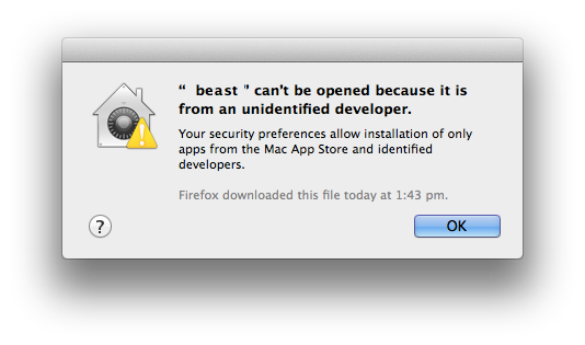
(Had to doctor this screenshot a bit to show beast instead of the app I started). Again, change the security settings (temporarily) to allow applications from anywhere, as outlined above.

Need to install Java 6?

Now the dmg file should open and you can drag BEAST to the Applications folder. Double clicking BEAUti or BEAST may result in a message asking you to install Java 6. This may seem strange if you already have Java 7 or higher installed.

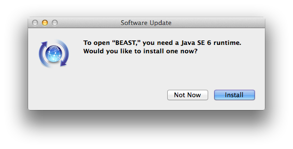
It does not change your default Java installation if you click ‘install’ — Java 6 will be installed next to Java 7 or 8, but will not become the default for command line usage.
(you may want to create a symbolic link to trick OSX in thinking Java 6 is already installed if you already have Java 7 — details here).

BEAST does not start from the command line

When you run BEAST or BEAUti from the command line, you can be confronted by a somewhat mysterious message like this:

Exception in thread "main" java.lang.UnsupportedClassVersionError: beast/app/beauti/Beauti : Unsupported major.minor version 52.0

BEAST v2.1.x requires Java 6 and v2.2.x requires Java 8. It is possible that you do not have the correct version of Java installed. To test which version you have, in a terminal use “java -version”, which should display something like this:

~> java -version
java version "1.8.0_11"
Java(TM) SE Runtime Environment (build 1.8.0_11-b12)
Java HotSpot(TM) 64-Bit Server VM (build 25.11-b03, mixed mode)

(~> is the command prompt, and should not be typed. Anything with out ~> is output to screen.) If you do not have the correct Java version installed, you can do so from java.com or for Java 8 oracle. It is possible that you have more than one version of Java installed, and that the default version happens to be an older version. To change the default version is a bit fiddly, but can be done from a terminal by changing a symbolic link in /System/Library/Frameworks/JavaVM.framework/Versions/ like so:

~> cd /System/Library/Frameworks/JavaVM.framework/Versions/
~> ls
CurrentJDK

If it shows something else, e.g., Current replace CurrentJDK with the name of that link.

~> rm CurrentJDK
~> ls /Library/Java/JavaVirtualMachines/
jdk1.7.0_21.jdk     jdk1.8.0_11.jdk

Now, just select one of the Java versions, say jdk1.8.0_11.jdk and add the link

~> ln -s /Library/Java/JavaVirtualMachines/jdk1.8.0_11.jdk/Contents/ CurrentJDK

Don’t forget to replace CurrentJDK with Current if that is what you had before.

BEAGLE and CUDA

BEAGLE is a library for performing Felsenstein’s peeling algorithm much more efficiently than can be done in Java. To install it for Mac is straightforward, but sometimes it does not work. One of the reasons is that the BEAGLE installer makes it easy to let you install CUDA as well. The CUDA library is useful only when you have an NVIDA graphics card. Most Macs that I’ve seen do not have an NVIDIA card, and on these machines you can see errors similar to this:

CUDA error: "Driver not initialized" from file , line 169.

What you need to do is uninstall the CUDA driver — reinstalling the BEAGLE library may be helpful as well.

Uninstalling CUDA drivers is a bit of a mission, since files go in a number of places, and there is no uninstaller. What should work is to delete all of the following files

/Library/Frameworks/CUDA.framework
/Library/LaunchAgents/com.nvidia.CUDASoftwareUpdate.plist
/Library/PreferencePanes/CUDA Preferences.prefPane
/System/Library/Extensions/CUDA
/System/Library/StartupItems/CUDA
/usr/local/cuda/lib/libcuda.dylib

then reboot, and CUDA should be uninstalled.

Accessing packages

BEAST packages typically come with usefule examples and documentation. On OSX, packages are stored in ~/Library/Application Support/BEAST/2.1/ and each package has its own directory with the name of the package. The OSX Finder does not show the ~/Library folder by default. To open the folder, click the Go-item in the menu bar, then hit the alt-key. Now ‘Library’ appears under the Go-menu. Select the Library-item and a new folder opens from where you can browse to the BEAST package.

Blog

BEAST Apps for the AppStore

August 4, 2014 rbou019 Leave a comment

4 August 2014 by Remco Bouckaert

Say, you have some post-processing classes written for your package and you want to make it available to users. Since the class is in your package, say mypackage.addon.jar and most likely you need classes from BEAST-core or other packages, it is a nuisance to set the class path from the command line. You’ll and up having to do something like

java -cp /path/to/beast/lib/beast.jar:~/.beast/2.1/MyPackage/lib/mypackage.addon.jar beast.app.tools.MyTool arg1 arg2 arg3

This is especially cumbersome to explain to users since these paths depend on where BEAST is installed and where packages are installed. These paths are operating system dependent. One solution to this is to use the BEAST AppStore. This is an application that comes with BEAST. It picks up information from the version.xml file. You specify an addonapp element with a description, class, default arguments and an icon. For example, the model-selection package contains an application to run a path sampling analysis, which is encoded like so:

When you start the AppStore, it will look like this:

If you launch it from the AppStore, you probably want to launch it as a GUI, since Windows and Mac users won’t be able to see any terminal input otherwise. You can write your own GUI in Swing or JavaFX if you like, but there are a few helper classes that make it very easy to write GUI applications with BEAST. The recipe is as follows:

Create a class for your App that derives from beast.core.Runnable.
Specify Inputs for each of the arguments for your application.
Implement the run() method to pick up values from inputs and run your app.
Create a class to launch the App.
Update the version.xml file

Path sample analyser application

Step 1: create class for App

The path sample analyser lives in the class beast.inference.PathSampleAnalyser and derives from beast.core.Runnable.

@Description("Reads logs produces through PathSampler and estimates marginal likelihood")
public class PathSampleAnalyser extends beast.core.Runnable {
}

Step 2: specify inputs

For the path sample analyser, we need a root directory, alpha, number of steps and burnin as a percentage. So, we add the following Inputs to the class.

public Input rootDirInput = new Input("rootdir", "root directory for storing particle states and log files (default /tmp)", "/tmp");
public Input alphaInput = new Input("alpha", "alpha parameter of Beta(alpha,1) distribution used to space out steps, default 0.3" +
		"If alpha <= 0, uniform intervals are used.", 0.3);
public Input stepsInput = new Input("nrOfSteps", "the number of steps to use, default 8", 8);
public Input burnInPercentageInput = new Input("burnInPercentage", "burn-In Percentage used for analysing log files", 50);

Step 3: implement `run()` method

The actual post-processing happens in the method estimateMarginalLikelihood. The run method just gather info from the inputs and passes it to that worker method.

@Override
public void run() throws Exception {
    // do the work
    double marginalL = estimateMarginalLikelihood(
			stepsInput.get(), 
			alphaInput.get(), 
			rootDirInput.get(), 
			burnInPercentageInput.get());

	// report the result       
	System.out.println("marginal L estimate = " + marginalL);
}

Step 4: Create launcher class

Create a class to launch the App. This is the class that you register in the version.xml file. The following bit of code can be used as a template for your own app — just replace the class for the analyser variable and update name and title. It uses two utility classes beast.app.util.Application and beast.app.util.ConsoleApp (currently in the model-selection package, but it should probably move somewhere else). You can also suppress inputs that you do not want to expose to the user.

package beast.app.tools;

import beast.app.beauti.BeautiConfig;
import beast.app.beauti.BeautiDoc;
import beast.app.draw.BEASTObjectDialog;
import beast.app.draw.BEASTObjectPanel;
import beast.app.util.Application;
import beast.app.util.ConsoleApp;

//command line interface to PathSampleAnalyser
public class PathSampleAnalyser {
		
	public static void main(final String[] args) throws Exception {
		Application main = null;
		try {
			// create the runnable class with application that we want to launch
			beast.inference.PathSampleAnalyser analyser = new beast.inference.PathSampleAnalyser();
			
			// need to set the ID of the BEAST-object
			analyser.setID("PathSampleAnalyser");
			
			// then initialise
			analyser.initAndValidate();
			
			// create BeautiDoc and beauti configuration
			BeautiDoc doc = new BeautiDoc();
			doc.beautiConfig = new BeautiConfig();
			doc.beautiConfig.initAndValidate();

			// This is how you suppress an input that we don't want to expose to the user
			// doc.beautiConfig.suppressPlugins.add(analyser.getClass().getName() + ".input-name");

		
			// create panel with entries for the application
			BEASTObjectPanel panel = new BEASTObjectPanel(analyser, analyser.getClass(), doc);
			
			// wrap panel in a dialog
			BEASTObjectDialog dialog = new BEASTObjectDialog(panel, null);
			if (dialog.showDialog()) {
				dialog.accept(analyser, doc);
				analyser.initAndValidate();

				// create a console to show standard error and standard output
				analyser.consoleApp = new ConsoleApp("PathSampleAnalyser", // name 
						"Path Sample Analyser: " + analyser.rootDirInput.get() // console title
						);

				analyser.run();
			}
		} catch (Exception e) {
			System.out.println(e.getMessage());
			if (main != null) {
				System.out.println(main.getUsage());
			}
		}
	}

}

Update the `version.xml` file

Add an addonapp element to the version.xml file, so the AppStore can pick it up.

When launching the PathSampleAnalyser from the AppStore, it looks like this:

Blog

All about starting trees

July 28, 2014 rbou019 Leave a comment

28 July 2014 by Remco Bouckaert

Before starting an MCMC run, BEAST uses State Node initialisers to set up the starting trees (and other parameters). Often a good starting tree is already available from another analysis (e.g. a maximum likelihood tree). Though it is against the spirit of MCMC, which guarantees any random starting state will lead to convergence, a good starting tree can help with large analysis to speed up convergence quite a bit. Of course another reason to specify a starting tree is if you want to do an analysis using just a single known tree topology.

We start with standard analysis, but see below for *BEAST analyses.

Standard analysis

For a standard analysis, there are three ways to specify a starting tree

a random tree
a tree in Newick format
a cluster tree, e.g. through UPGMA or neighbour joining

By default, BEAUti uses a RandomTree state-node initialiser to generate a starting tree. If you want to replace it with a Newick tree or cluster tree, first you need to remove (or comment out) the RandomTree element from the XML. For a tree in partition XYZ26, just search for RandomTree and remove the XML fragment with id RandomTree.t:XYZ26. It should look something like this:

1.0

Before removing, make note of the initial attribute (@Tree.t:XYZ26> here) and taxa attribute (@XYZ26 here).

Newick starting tree

After removing the Random tree, in the same place, add a TreeParser using the following fragment

The attributes that you want to specify are

id="NewickTree.t:XYZ26" the ID should be unique, so something like NewickTree.t: plus the name of the tree would be suitable.
initial="@Tree.t:XYZ26" this refers to the tree being initialised. It should be the same as the initial attribute of the RandomTree that was removed.
taxa="@XYZ26" this refers to the alignment and ensures that taxa in the tree are lined with those in the alignment. For BEAST v2.1.x, this must be specified to prevent starting with a mislabelled tree
newick="((your,(tree,goes)),here)" obviously needs to be replaced with your own tree in Newick format.

This is all you need to know to set up a starting tree. There are a few optional attributes you can use to make life a bit easier:

adjustTipHeights is true by default, which means tips of the tree will be set to zero, or if tip dates are specified to these particular tip dates. By setting to adjustTipHeights="false", tips will be initialised by the heights in the Newick tree.
if adjustTipHeights="false" then threshold specifies threshold under which node heights (derived from lengths) are set to zero. This helps when there are numeric issues with adding the lengths.
scale scale used to multiply internal node heights during parsing. Useful for importing starting from external programs, for instance, RaxML tree rooted using Path-o-gen.
IsLabelledNewick="true" Is the Newick tree labelled (alternatively contains node numbers)?
If sLabelledNewick="false" then “offset="1" is the lowest taxa number. The default=1 but 0 is common as well. Taxa numbers are as they are ordered in the alignment referred to with the taxa attribute.

Cluster tree

After removing the Random tree, in the same place, add a ClusterTree with the following fragment

The attributes that you need to specify are id='UPGMATree.t:XYZ26', initial="@Tree.t:XYZ26" and taxa="@XYZ26", which are as for Newick tree (see above).

You can use different clustering algorithms by specifying the clusterType="upgma" attribute.

clusterType	Description
single	single link
complete	complete link
upgma or average	UPGMA=average link
mean	mean link
centroid	centroid
ward	Ward’s method
adjcomplete	adjusted complete link
neighborjoining	neighborjoining
neighborjoining2	neighborjoining2 – corrects tree for tip data, unlike plain neighborjoining

*BEAST analysis

For a *BEAST analysis, the default in BEAUti is to generate a UPGMA tree for the species tree, then generate UPGMA trees for each of the gene trees and fit them inside the species tree. In previous incarnations of BEAST, a random tree was generated for species as well as for gene trees, but gene tree branches ending in leaves were lengthened such that each first coalescence of a gene tree was above the root of the species tree. Though this ensures that the gene trees fit inside the species tree, it leads to long burn-in times.

If you want to use a different starting tree for the species tree, first move (not remove!) the StarBeastStartState element generated by BEAUti to just before the run-element with id="mcmc". BEAUti will have generated some elements inside the start-state (such as the species-tree-prior) that we need elsewhere in the analysis. By moving the init element outside the run element, it will not activate the StarBeastStartState.

The StarBeastStartState looks something like this:

For every gene tree there will be a tree entry in the StarBeastStartState. To replace the species tree with a Newick tree, add the following fragment (at the place where the StarBeastStartState was):

The only thing to set up is the Newick using the newick attribute — all other attributes should be as they are (it is using the species tree, which is identified by the Species partition in every *BEAST analysis generated by BEAUti).

For each of the gene trees, you need to specify a tree as well. You can specify them using a Newick tree as for the Standard analysis (see above). Alternatively, you can use a random tree that is placed ‘above’ the species tree. To do this, you add for the first gene tree (just below the new Species tree start tree):

where you replace the initial='@Tree.t:26' and taxa="@26" attributes to match your tree (instead of 26, as in this example). For every subsequent gene tree, you add (below the first gene start tree):

where you replace the initial='@Tree.t:29' and taxa="@29" attributes to match your tree (instead of 29) and make sure the id is unique.

Tip calibration in BEAUti

Tip calibration in XML

Tip sample operator in XML

Add logger entry

Bayes factor delimitation

Threshold based methods DISSECT/STACEY

Links

Package added since the last udpate on this blog

MGSM: multi-gamma site model

Spherial geography

bModelTest

Morphological-models

Sampled ancestors

The coalescent SIR model

Metroplolis coupled MCMC

Species delimitation with DISSECT and STACEY

Bayesian structured coalescent approximation with BASTA

More tutorials

Why use sampled ancestor trees instead of binary trees?

Tree priors for sampled ancestor trees

Setting up an analysis

The coalescent SIR model

Using the model in XML

The stochastic coalescent SIR model

Coming up

DMG is ‘damaged’

Cannot be opened

Need to install Java 6?

BEAST does not start from the command line

BEAGLE and CUDA

Accessing packages

Path sample analyser application

Step 1: create class for App

Step 2: specify inputs

Step 3: implement run() method

Step 4: Create launcher class

Update the version.xml file

Standard analysis

Newick starting tree

Cluster tree

*BEAST analysis

Bayesian evolutionary analysis by sampling trees

Step 3: implement `run()` method

Update the `version.xml` file