BEAUti

BEAUti now allows imports of calibrations from NEXUS files, so you can specify tip dates, distributions on tip dates, monophyletic constraints and clade calibrations in a NEXUS file. This is especially handy when there are a large number of calibrations or when a large number of clades need to be defined.

BEAUti now has a “File/Launch Apps” menu to start applications provided by packages, such as the GUI for doing a Path Sampling analysis (as the AppStore does).

In Windows and Linux, the *BEAST template went missing at the second time BEAUti was started due to a bug in the way packages are handled. This is fixed now.

Streamlined upgrades of BEAST so when you can upgrade BEAST as simple as upgrading any package. When upgrading BEAST, BEAUti exits and when restarting it downloads the latest version — which may take a little time.

BEAST

On OSX, a common problem was that a CUDA driver was installed to support BEAGLE, but that there is no hardware that is CUDA enabled. The result was a crash of BEAST without an error message, which made it hard to find out what went wrong. In this version a test is done for this condition, and if it exists, instructions are provided on how to uninstall CUDA drivers, which should fix the problem.

The CLI script for BEAST should have less trouble loading the BEAGLE library in Linux and OSX.

Two operators have improved operator tuning resulting in slightly better performance (higher ESSs) in most cases.

There are some improvements in reporting error conditions, which should help diagnose problems.

LogAnalyser

A bug crept into v2.4.0 causing LogAnalyser not to show progress on loading and processing the log file when started from CLI, which is fixed now.

March 2016 by Remco Bouckaert, Tim Vaughan, Walter Xie, and Alexei Drummond

Recently, a few users reported problems with BEAST 2 performance, concluding it was worse than BEAST 1. This puzzled us, because BEAST 1 and 2 share the same core algorithms, and both spend most of their time doing phylogenetic likelihood calculations, which is optimised using BEAGLE, a library shared by both programs. In fact, recently we changed the way that BEAST 2 handles proportion invariant categories, saving some phylogenetic likelihood calculations, so in theory it should be faster when using a proportion of invariant sites in the model. So, we became curious whether there are real performance differences between BEAST 1 and 2 and decided to do a benchmark. We expected them to perform roughly the same on GTR and GRT+G analyses, and BEAST 2 to do better on GTR+I and GTR+G+I analyses.

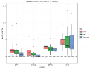
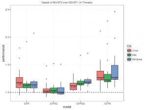
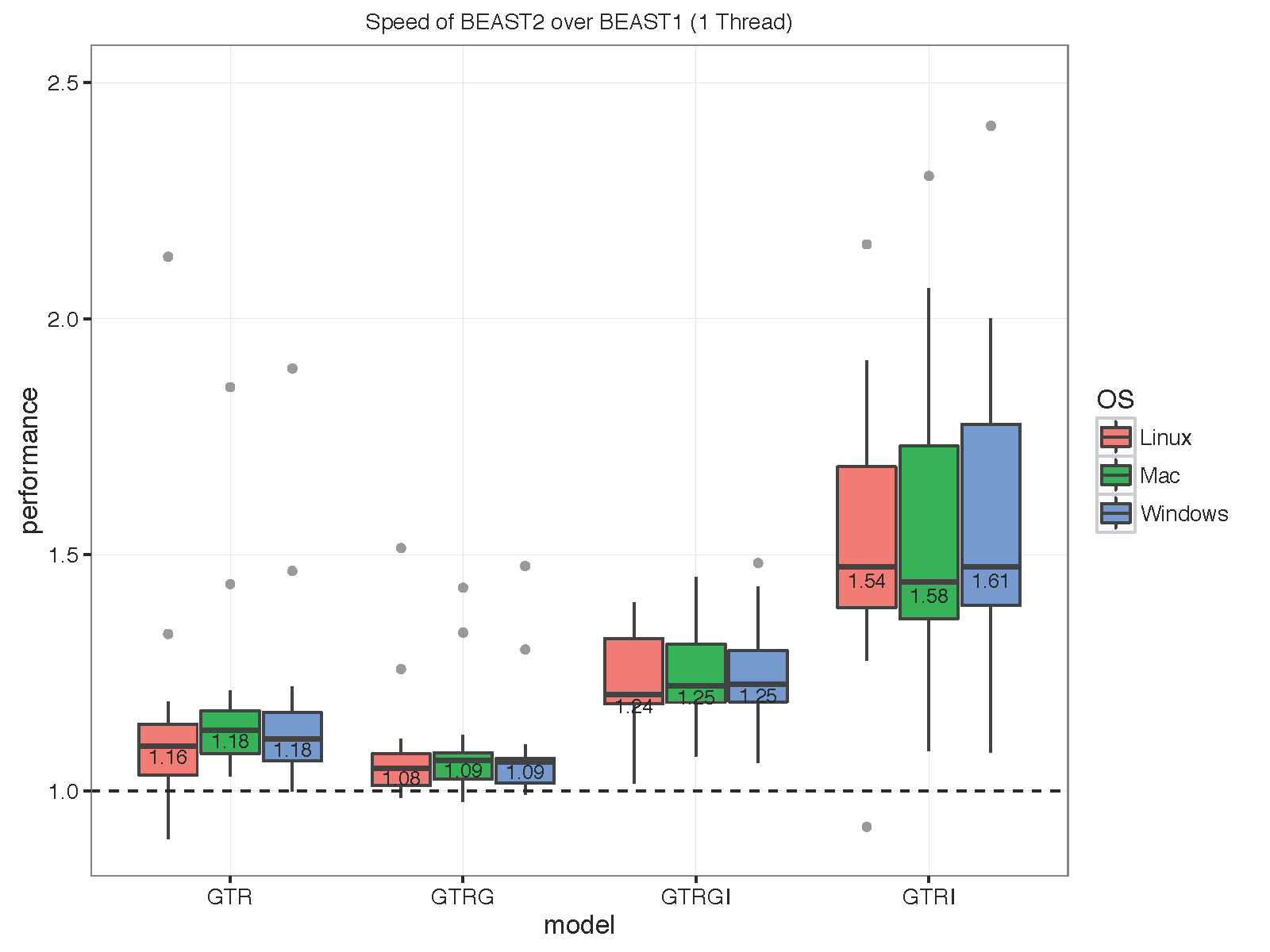
The picture below summarises the speed of BEAST 2 over BEAST 1 using 1, 2, 4 thread(s) in the 3 different operation systems. As you can see the performance is very similar for GTR and GTR+G, with BEAST2 being perhaps slight faster (although this could be due to debugging that BEAST1 performs at the start of the chain):

What we did

Analyses

BEAST can do many kinds of analyses, but for the purpose of this benchmark, we want to see whether the TreeLikelihood calculations, which typically dominate the computational time of MCMC runs, are comparable. To see the impact of the way BEAST 2 handles proportion invariant, we want to have an analysis with and without a proportion invariant category. And since many analyses use gamma rate heterogeneity with and without proportion invariants, we end up with four variants:

• GTR
• GTR + 4 gamma categories
• GTR + proportion invariant
• GTR + 4 gamma categories + proportion invariant

To keep things otherwise simple, we use a Yule tree prior, a strict clock and start with a random tree. To be practical, we set up the analysis in BEAUti 1 and 2, just importing an alignment, choosing the site model, setting the tree prior in BEAST 1 (BEAST 2 uses Yule by default) and save to file. As it turns out, the analyses produced that way are almost the same, but there are some small differences in the operator settings. Due to auto-optimisation, they will eventually become almost the same, but to make the two analyses as equal as possible we edited the XML so that they have the same operator weights and tuning values. Also, the population size used to generate the random starting tree differed so these were made the same as well.

The MCMC runs were run for 1 million steps in order to make them long enough that the slightly different ways extra likelihood calculations are done at the start for debugging purposes has little effect on the outcome. Also, with longer runs JIT compiler differences are eliminated. We took care to run the different programs under the same circumstances, on a computer not doing any other jobs at the time.

This whole process was automated to deal with the various data sets we wanted to test.

Threading

The way to set up threads in BEAST 2 is a bit cumbersome (v2.4.0 improves things a lot), so perhaps the reason is different configurations of threading. Therefore, we want to see what the impact of threading is. That led us to 3 variants:

• 1 thread BEAGLE SSE
• 2 thread BEAGLE SSE
• 4 thread BEAGLE SSE

For BEAST 1, we used the flags -overwrite -beagle_instances. For BEAST 2 we used -overwrite -threads for the SSE runs. For all cases, we verified that both programs use the same settings of BEAGLE as reported at the start of the run.

Data sets

To get an impression of the impact of different data, we randomly selected a number of data sets from treebase.org with a number of sizes. We also used the data sets from the BEAST 1 examples benchmark directory giving a total of 15 data sets.

Versions

To have a fair comparison, we used the latest versions currently avaiable v1.8.3 and v2.4.0.

Results

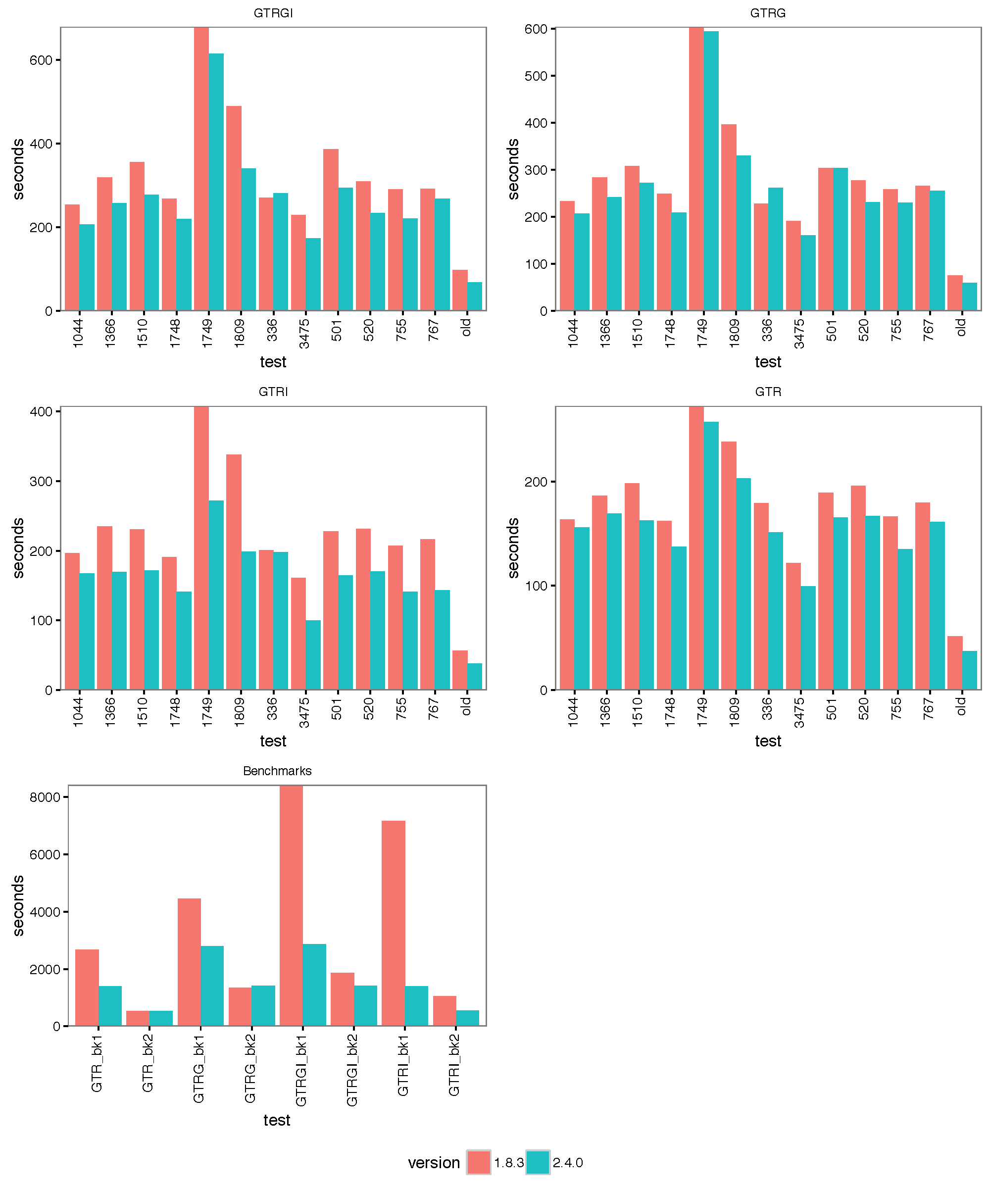
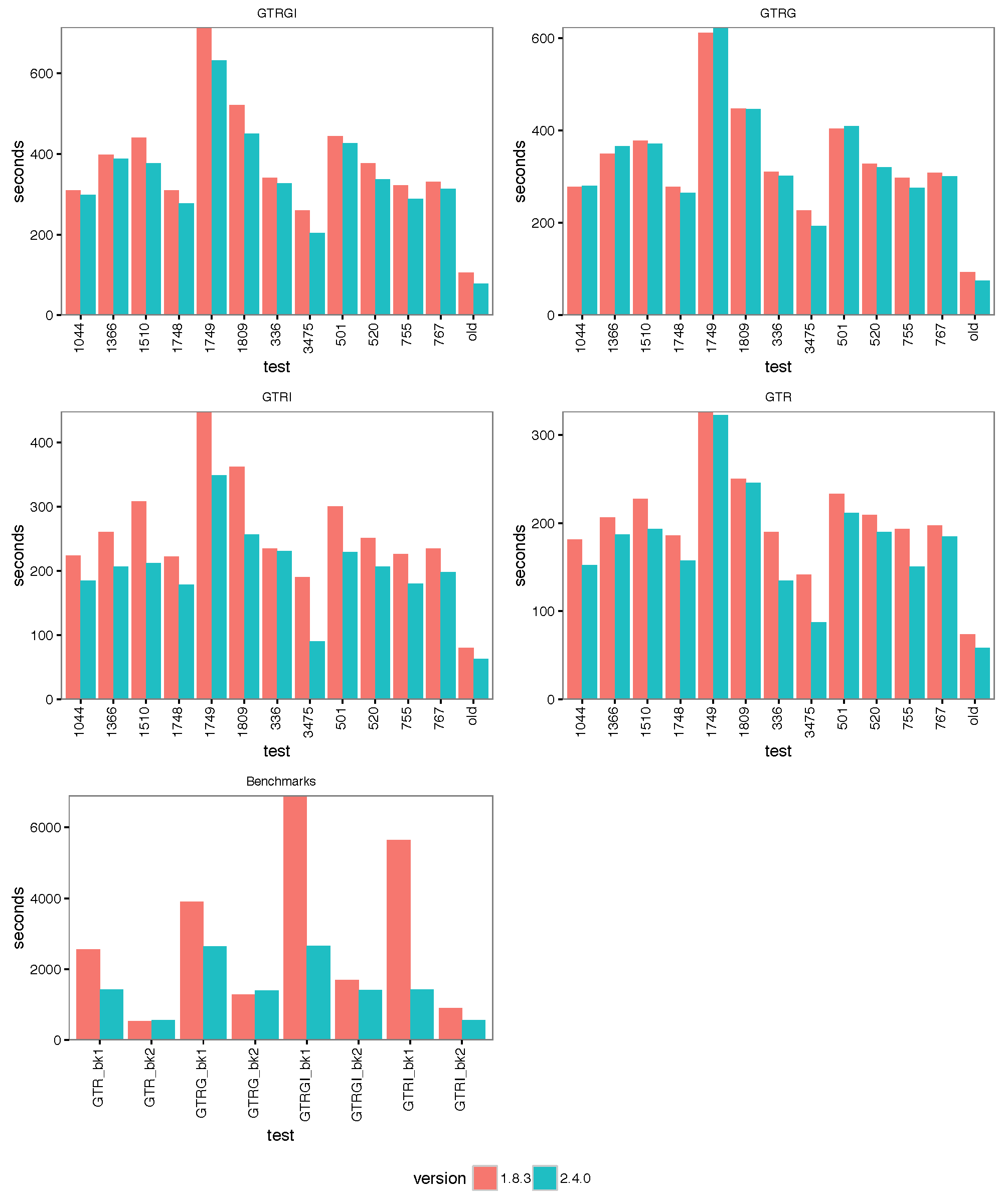
The images below show the run time for 1, 2, 4 thread(s) in Linux, where 1.8.3(t0) presents no threading pool for single thread in BEAST 1.8.3.

• 1 thread:
  
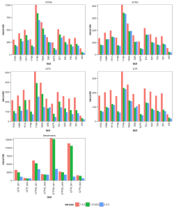
• 2 threads:
  
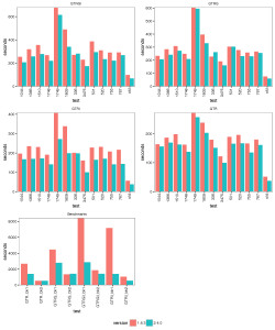
• 4 threads:
  

With increasing number of threads, the difference in run time in seconds decreases, but BEAST 2 is almost always slightly faster than BEAST 1 in these comparisons. However, it turned out that the data sets are too small for four threads to be of much use — the four threaded runs tended to be slower than for two threads, which is optimal for most of these datasets for both BEAST versions. This may also be a function of the hardware used.

Cursory checks of ESSs for BEAST 1 and 2 in Tracer did not show any substantial difference, which is not surprising since the same mixture of operators was used. Also, parameter estimates tended to agree between some randomly selected analyses.

To make sure that it differences are not OS dependent, we ran the analyses on Windows 7, OS X and Linux, but did not find any substantial differences between the operating systems.

Conclusions

To our surprise, we found that BEAST 2 is slightly faster than BEAST 1. This is not what we expected since both programs perform the same analysis using the same BEAGLE library. Although we did our best to compare apples with apples, it is possible we overlooked something, so let us know if you find anything that can explain the differences in performance.

If you want to replicate these runs, you can find them in the benchmark repository on https://github.com/CompEvol/benchmark, which includes the data, some instructions and scripts to run them.

BEAST improved performance

BEAST is up to 2x faster when using proportion invariant sites and BEAGLE. When using proportion invariant in combination with gamma rate heterogeneity, it still is faster than before.

BEAST always had a “beagle_instance” command line flag, that was essentially ignored. This is now replaced by an flag that actually works, and is named “instances” since it works both with java and BEAGLE tree likelihoods.

By default, the treelikelihood is now threaded for analyses using the Standard template in BEAUti. The number of threads used per treelikelihood is determined by the “instances” flag, but can be overridden using the “threads” attribute of ThreadedTreeLikelihood (which was migrated from the BEASTLabs package).

Further, there are a few minor performance improvements, including faster MRCAPrior handling.

A bug in StartBeastStartState was fixed to work with calibrations with other than the CalibratedYule prior.

BEAUti

The parametric distributions in priors panel now show mean as well as median of the distribution.

There is better taxon management preventing adding numbers to taxon names

The layout tip dates panel was improved to deal with changing window sizes.

A bug in *BEAST clock cloning is fixed.

Allow setting branch length as substitution option on tree logger, which was previously not possible.’

Improved JSON export of BEAST analyses (just use json as extension to the file when saving) and using a library with a more sensible license.

Package manager

The package manager has been changed so it can read all package information (including that of older versions) from a single package file. A bigger change is that BEAST is now treated as a separate package: when you start any of the BEAST applications, it loads the beast.jar file from the user package directory, and if it is not already there, will put a copy in that place. This makes it much easier to upgrade BEAST: just select BEAST in the package list and click the install/update button.

The GUI of the package manager is improved, among other things, showing by colour whether a package can be installed.

For developers

The biggest change with this release is really for developers, as outlined in a separate post here.

Packages

Due to some API changes, all packages have been re-released. Some packages have not been updated yet, but will be soon. New packages expected soon that have not been available before include startbeast2 and correlated characters.

3 February 2016 by Remco Bouckaert

Most significant upcoming changes are

• Annotated constructor support, so instead of using Input and initAndValidate you can use constructors and use most of the info that now goes into and Input in a @Param annotation. See, for example AnnotatedRunnableTestClass and JSONTest.
• Better JSON support for BEAST specifications, using a non-evil JSON library.
• Removal of Exceptions in favour of classes that derive from Exception. This means that many methods that previously were throwing Exceptions, are throwing more specialised Exceptions, or nothing at all (if only RuntimeExceptions are thrown).
• Cleaned up code, better conforming to Java 8 constructions and naming conventions. Also, attempt to remove the term ‘Plugin’ and replace with BEAST object where appropriate, since the term plugin is not used any more.

Code changes

This is a (still evolving) list of changes for package developers containing possible changes required to make packages compatible with BEAST v2.4.0. Mostly, there are minor method signature changes, and some member variables name changes, with the exception of Exceptions.

Exceptions

However, the biggest change is that throws Exception on initAndValidate will be removed. initAndValidate is supposed to check validity of values of inputs, and initialise. If for some reason this fails, the most appropriate exception to throw is IllegalArgumentException or RuntimeException.

Note you can always throw fewer exceptions than the method derived from, so you can change your code to work with both v2.3 and v2.4 by just removing or specialising the exception that is thrown.

Signature changes

The signature of BeautiDoc.deepCopyPlugin changes: requires an extra argument to tell which partition to copy from.

Access changes

A number of package private member and methods now are protected to allow access from difference packages.
BeautiAlignmentProvider.getAlignments(),

Most inputs are now final, so cannot be re-assigned.

Name changes

SubtreeSlide.fSize is now SubtreeSlide.size
InputEditor.m_plugin is now InputEditor.beastObject
BeautiConfig.inlinePlugin, collapsedPlugins, suppressPlugins are now inlineBEASTObject, collapsedBEASTObjects, suppressBEASTObjects

Deprecated

BEASTObject.outputs is now private. Use BEASTObject.getOutputs() to access the set of outputs.

Main reason for this release is to get the path corrected so Standard and StarBeast templates are visible under templates menu. In the v2.3.1 they got lost due to a new way of handling search paths. But there are many other reasons to upgrade to this release as pointed out below.

BEAUti

A fix of import of traits from file when partitions are split into say codon positions.

A fix for cloning of scripts with partition information.

Set up weights correctly of FixedMeanRate operator when ascertainment correction is applied. Previously, ascertainment correction columns were included in the weights.

Allows ParameterInputEditor to edit Parameter inputs.

Ensure when focus is on an editable field in Taxon set dialog the last value entered is captured when switching tabs.

BEAST

A “-validate” command line option for was added for parsing XML files without running them. This can be useful for just testing whether an XML file is correct, without having to stop the MCMC run and delete log files that are being created.

The MRCAPrior is now much more efficient. This gives performance improvements when there is little data and many MRCAPriors.

The way of generating random trees has been robustified.

More robust storing the state file on Windows.

LogCombiner

Ensured in the GUI version of LogCombiner burn in editing finished properly. The burn in was previously ignored if the burn in field was edited and the focus left on the edit field when pressing the run button.ds

LogAnalyser

LogAnalyser now has one line per file mode, so you can analyse multiple files and instead of having all info printed as blocks it can output all results for a single log file on a single line. This is handy when importing in R for further post-processing.

A CLI script added in the bin directory for ease of launch.

Error messages

More sensible error messages in many classes, for instance TreeParser, RPNCalculator, NodeReheight.

DensiTree is updated to version 2.2.4.

Packages

New releases of the following packages were created since the release v2.3.1:
* BACTER,
* GEO_SHERE,
* STACEY,
* bModelTest,
* SNAPP,
* BASTA,
* RBS.
* MultiTypTree and
* MASTER.

BEAUti fixes

Robustify (un)linking of partitions.

Improved Fasta import.

BEAST

Support for probability vectors for uncertain sequences (see examples/testJukesCantorShortUncertain.xml), which are alignments where characters are encoded as a distribution.

Improved error messages.

TreeAnnotator

TreeAnnotator has a flag to make it use less memory. The original implementation loaded all trees in memory, which could take up quite a bit of space, especially because the default memory limits were set to 1GB (now increased to 4GB). Setting the flag causes TreeAnnotator not to load the whole tree set in memory, just a single tree at the time.

TreeAnnotator now recognises -b as flag to specify burn-in.

AppStore, LogCombiners, LogAnalyser

Command line interface are improved for these applications. Use application -help to see details.

Misc

Tree parsing is now based on Antlr instead of a hand crafted parser.

DensiTree updated to v2.2.3.

BinaryCovarion model option to run as reversible model. The original implementation did not take the hidden frequencies in account when setting up the rate matrix, resulting in an irreversible model in case the hidden frequencies deviated from (0.5, 0.5). Set the mode="REVERSIBLE" attribute in the XML to make it do so.

Set log level by environment variable. There are five log-levels (error, warning, info, debug, trace) which from left to right log increasingly more information. Only BEAST has a flag to set the level, but other applications do not. Now, you can set an environment variable beast.log.level to the desired value. Either set it external variable, e.g. export beast.log.level=debug on Linux, or add as directive to java through java -Dbeast.log.level=debug -cp beast.jar .....

BASTA

A package for approximate structured coalescent, now allows Bayesian stochastic variable selection.

BACTER

A package providing limited support for ancestral recombination graphs a la ClonalOrigin, but with all the substitution models and other support provided by BEAST.
Documentation here.

BEASTLabs

More efficient handling of many monophyletic constraints through the MultiMonophyletic prior

A few operators were added to deal with multiple monophyletic constraints, including restricted subtree slide (RestrictedSubtreeSlide), restricted nearest neighbour interchange (NNI), and restricted subtree prune regraft (SPR).

Others

Many refinements in other packages were made as well, so upgrading to the latest version will be worth it.

7 July 2015 by Remco Bouckaert

These are a few issues that can pop up when doing ancestral reconstruction aka discrete phylogegraphy as outlined in the Ancestral reconstruction tutorial following the model of Lemey et al, 2009.

Too many states

When doing a phylogeographical analysis, it is tempting to split up the samples in as fine a geographic classification as the available data allows — for instance by splitting the samples by country of origin. This can lead to a large number of states/countries. The more states are defined, the more rates need to be estimated. For an analysis with N states, at least N-1 rates need to be specified in order to be able to get from any one state to any other (possibly through a set of other states), and this is a requirement for the likelihood to be larger than zero.

So, it depends on the number of samples what a reasonable number of states can be; more samples allow for more states. I have seen a number of cases where it was attempted to use a number of states more than half the number of states. In such cases, it makes sense to merge states (combine different countries into larger regions)

Note that ancestral reconstruction has no notion of how far samples are apart from each other, so it can only estimate rates based on state transitions in the tree informed by locations at the tips. Instead of using ancestral state reconstruction, you could use a form of continuous phylogeography, which tends to have more power since it has a notion of distance built in. If you do not know the exact point locations of the tips, tip locations can be sampled, or approximated by the mean of the region where the sample originated.

Analysis does not start

A common result of defining too many states is that the analysis does not start. You will see an error containing something like this:

Start likelihood: -Infinity after 11 initialisation attempts
P(posterior) = -Infinity (was NaN)
	P(prior) = -Infinity (was NaN)
		P(CoalescentConstant.t:chr1) = -224.91126226515757 (was NaN)
		P(GammaShapePrior.s:chr1) = -1.0 (was NaN)
		P(KappaPrior.s:chr1) = -1.8653600339742873 (was NaN)
		P(nonZeroRatePrior.s:location) = -Infinity (was NaN)
		P(PopSizePrior.t:chr1) = 1.2039728043259361 (was NaN)
		P(relativeGeoRatesPrior.s:location) = -350.99999999999994 (was NaN)
		P(geoclockPrior.c:location) = -6.915086640662835 (was NaN)
	P(likelihood) = NaN (was NaN)
		P(treeLikelihood.chr1) = NaN (was NaN)
		P(traitedtreeLikelihood.location) = NaN (was NaN)

Note the Infinity in the line for nonZeroRatePrior.s:location. This is the prior over the number of rates that are used. By default, this prior is a Poisson prior with mean of 0.693 and offset equal to the number of states minus 1. This is a rather tight prior. At the start, by default all rates are estimated. And though in theory the Poisson prior extends over the range of positive numbers, due to numerical issues, the probability of the number of estimated rates can be large enough that the support can become zero.

Workarounds for this are

• Reduce the number of states.
• Start with a wider prior on non-zero rates by increasing the value of lambda, or use a different prior altogether. Once the analysis runs for a little while you can stop it, set the prior back and resume.
• Set up a start state that contains more zeros. This is a bit fiddly, since it involves editing the XML. Find the rateIndicator parameter ( id="rateIndicato.s:location"). Its value say is true, and it has dimension N. For parameters that have less values than the dimension its value is copied till all N values are available. So, if you have dimension=6 (i.e., we need 6 flags) and value=”true false” it will be copied 3 times, giving “1 0 1 0 1 0″. With value=”true false true” we get “1 0 1 1 0 1”.
  So, what you can do if you have N states is set up a set of values such that only the N-1 rates along the diagonal are true.

Analysis does not converge

There are many reasons an analysis does not converge (there are several sections on it in the book and tips on how to increase ESS). Probably, the first you want to do is make sure rates are set up correctly.

A specific reasons for the ancestral state reconstruction to fail include that there are too many states, hence there is not enough data for the rates to be estimated.

Numeric instability with asymmetric analysis

By default, the ancestral reconstruction uses a symmetric rate matrix, like her on the left.

By setting the symmetric attribute to false on the element with spec="SVSGeneralSubstitutionModel", an asymmetric rate matrix is used, which means going from state 1 to 2 can get a different rate than the other way around. This means that potentially the number of rates is doubled. It also means that the rateindicator has a dimension that is doubled.

This can lead to numeric instability for the eigensystem (which does an Eigen value decomposition of the rate matrix), which means your analysis won’t start. This can be solved by changing the default Eigen-decomposition method to a more robust variant by setting the eigenSystem attribute of the substitution model to beast.evolution.substitutionmodel.RobustEigenSystem so the substitution model looks something like this:

    
        0.33333333333