All posts by rbou019

What is new in v2.4.0 and its packages — this site is deprecated: goto https://www.beast2.org/ for up-to-date information

BEAST improved performance

BEAST is up to 2x faster when using proportion invariant sites and BEAGLE. When using proportion invariant in combination with gamma rate heterogeneity, it still is faster than before.

BEAST always had a “beagle_instance” command line flag, that was essentially ignored. This is now replaced by an flag that actually works, and is named “instances” since it works both with java and BEAGLE tree likelihoods.

By default, the treelikelihood is now threaded for analyses using the Standard template in BEAUti. The number of threads used per treelikelihood is determined by the “instances” flag, but can be overridden using the “threads” attribute of ThreadedTreeLikelihood (which was migrated from the BEASTLabs package).

Further, there are a few minor performance improvements, including faster MRCAPrior handling.

A bug in StartBeastStartState was fixed to work with calibrations with other than the CalibratedYule prior.

BEAUti

The parametric distributions in priors panel now show mean as well as median of the distribution.

There is better taxon management preventing adding numbers to taxon names

The layout tip dates panel was improved to deal with changing window sizes.

A bug in *BEAST clock cloning is fixed.

Allow setting branch length as substitution option on tree logger, which was previously not possible.’

Improved JSON export of BEAST analyses (just use json as extension to the file when saving) and using a library with a more sensible license.

Package manager

The package manager has been changed so it can read all package information (including that of older versions) from a single package file. A bigger change is that BEAST is now treated as a separate package: when you start any of the BEAST applications, it loads the beast.jar file from the user package directory, and if it is not already there, will put a copy in that place. This makes it much easier to upgrade BEAST: just select BEAST in the package list and click the install/update button.

The GUI of the package manager is improved, among other things, showing by colour whether a package can be installed.

For developers

The biggest change with this release is really for developers, as outlined in a separate post here.

Packages

Due to some API changes, all packages have been re-released. Some packages have not been updated yet, but will be soon. New packages expected soon that have not been available before include startbeast2 and correlated characters.

What will change in v2.4.0 for developers — this site is deprecated: goto https://www.beast2.org/ for up-to-date information

3 February 2016 by Remco Bouckaert

Most significant upcoming changes are

  • Annotated constructor support, so instead of using Input and initAndValidate you can use constructors and use most of the info that now goes into and Input in a @Param annotation. See, for example AnnotatedRunnableTestClass and JSONTest.
  • Better JSON support for BEAST specifications, using a non-evil JSON library.
  • Removal of Exceptions in favour of classes that derive from Exception. This means that many methods that previously were throwing Exceptions, are throwing more specialised Exceptions, or nothing at all (if only RuntimeExceptions are thrown).
  • Cleaned up code, better conforming to Java 8 constructions and naming conventions. Also, attempt to remove the term ‘Plugin’ and replace with BEAST object where appropriate, since the term plugin is not used any more.

Code changes

This is a (still evolving) list of changes for package developers containing possible changes required to make packages compatible with BEAST v2.4.0. Mostly, there are minor method signature changes, and some member variables name changes, with the exception of Exceptions.

Exceptions

However, the biggest change is that throws Exception on initAndValidate will be removed. initAndValidate is supposed to check validity of values of inputs, and initialise. If for some reason this fails, the most appropriate exception to throw is IllegalArgumentException or RuntimeException.

Note you can always throw fewer exceptions than the method derived from, so you can change your code to work with both v2.3 and v2.4 by just removing or specialising the exception that is thrown.

Signature changes

The signature of BeautiDoc.deepCopyPlugin changes: requires an extra argument to tell which partition to copy from.

Access changes

A number of package private member and methods now are protected to allow access from difference packages.
BeautiAlignmentProvider.getAlignments(),

Most inputs are now final, so cannot be re-assigned.

Name changes

SubtreeSlide.fSize is now SubtreeSlide.size
InputEditor.m_plugin is now InputEditor.beastObject
BeautiConfig.inlinePlugin, collapsedPlugins, suppressPlugins are now inlineBEASTObject, collapsedBEASTObjects, suppressBEASTObjects

Deprecated

BEASTObject.outputs is now private. Use BEASTObject.getOutputs() to access the set of outputs.

What is new in v2.3.2 and its packages — this site is deprecated: goto https://www.beast2.org/ for up-to-date information

Main reason for this release is to get the path corrected so Standard and StarBeast templates are visible under templates menu. In the v2.3.1 they got lost due to a new way of handling search paths. But there are many other reasons to upgrade to this release as pointed out below.

BEAUti

A fix of import of traits from file when partitions are split into say codon positions.

A fix for cloning of scripts with partition information.

Set up weights correctly of FixedMeanRate operator when ascertainment correction is applied. Previously, ascertainment correction columns were included in the weights.

Allows ParameterInputEditor to edit Parameter inputs.

Ensure when focus is on an editable field in Taxon set dialog the last value entered is captured when switching tabs.

BEAST

A “-validate” command line option for was added for parsing XML files without running them. This can be useful for just testing whether an XML file is correct, without having to stop the MCMC run and delete log files that are being created.

The MRCAPrior is now much more efficient. This gives performance improvements when there is little data and many MRCAPriors.

The way of generating random trees has been robustified.

More robust storing the state file on Windows.

LogCombiner

Ensured in the GUI version of LogCombiner burn in editing finished properly. The burn in was previously ignored if the burn in field was edited and the focus left on the edit field when pressing the run button.ds

LogAnalyser

LogAnalyser now has one line per file mode, so you can analyse multiple files and instead of having all info printed as blocks it can output all results for a single log file on a single line. This is handy when importing in R for further post-processing.

A CLI script added in the bin directory for ease of launch.

Error messages

More sensible error messages in many classes, for instance TreeParser, RPNCalculator, NodeReheight.

DensiTree is updated to version 2.2.4.

Packages

New releases of the following packages were created since the release v2.3.1:
* BACTER,
* GEO_SHERE,
* STACEY,
* bModelTest,
* SNAPP,
* BASTA,
* RBS.
* MultiTypTree and
* MASTER.

What is new in v2.3.1 and its packages — this site is deprecated: goto https://www.beast2.org/ for up-to-date information

BEAUti fixes

Robustify (un)linking of partitions.

Improved Fasta import.

BEAST

Support for probability vectors for uncertain sequences (see examples/testJukesCantorShortUncertain.xml), which are alignments where characters are encoded as a distribution.

Improved error messages.

TreeAnnotator

TreeAnnotator has a flag to make it use less memory. The original implementation loaded all trees in memory, which could take up quite a bit of space, especially because the default memory limits were set to 1GB (now increased to 4GB). Setting the flag causes TreeAnnotator not to load the whole tree set in memory, just a single tree at the time.

TreeAnnotator now recognises -b as flag to specify burn-in.

AppStore, LogCombiners, LogAnalyser

Command line interface are improved for these applications. Use application -help to see details.

Misc

Tree parsing is now based on Antlr instead of a hand crafted parser.

DensiTree updated to v2.2.3.

BinaryCovarion model option to run as reversible model. The original implementation did not take the hidden frequencies in account when setting up the rate matrix, resulting in an irreversible model in case the hidden frequencies deviated from (0.5, 0.5). Set the mode="REVERSIBLE" attribute in the XML to make it do so.

Set log level by environment variable. There are five log-levels (error, warning, info, debug, trace) which from left to right log increasingly more information. Only BEAST has a flag to set the level, but other applications do not. Now, you can set an environment variable beast.log.level to the desired value. Either set it external variable, e.g. export beast.log.level=debug on Linux, or add as directive to java through java -Dbeast.log.level=debug -cp beast.jar .....

BASTA

A package for approximate structured coalescent, now allows Bayesian stochastic variable selection.

BACTER

A package providing limited support for ancestral recombination graphs a la ClonalOrigin, but with all the substitution models and other support provided by BEAST.
Documentation here.

BEASTLabs

More efficient handling of many monophyletic constraints through the MultiMonophyletic prior

A few operators were added to deal with multiple monophyletic constraints, including restricted subtree slide (RestrictedSubtreeSlide), restricted nearest neighbour interchange (NNI), and restricted subtree prune regraft (SPR).

Others

Many refinements in other packages were made as well, so upgrading to the latest version will be worth it.

Common problems with ancestral state reconstruction/discrete phylogeography in BEAST — this site is deprecated: goto https://www.beast2.org/ for up-to-date information

7 July 2015 by Remco Bouckaert

These are a few issues that can pop up when doing ancestral reconstruction aka discrete phylogegraphy as outlined in the Ancestral reconstruction tutorial following the model of Lemey et al, 2009.

Too many states

When doing a phylogeographical analysis, it is tempting to split up the samples in as fine a geographic classification as the available data allows — for instance by splitting the samples by country of origin. This can lead to a large number of states/countries. The more states are defined, the more rates need to be estimated. For an analysis with N states, at least N-1 rates need to be specified in order to be able to get from any one state to any other (possibly through a set of other states), and this is a requirement for the likelihood to be larger than zero.

So, it depends on the number of samples what a reasonable number of states can be; more samples allow for more states. I have seen a number of cases where it was attempted to use a number of states more than half the number of states. In such cases, it makes sense to merge states (combine different countries into larger regions)

Note that ancestral reconstruction has no notion of how far samples are apart from each other, so it can only estimate rates based on state transitions in the tree informed by locations at the tips. Instead of using ancestral state reconstruction, you could use a form of continuous phylogeography, which tends to have more power since it has a notion of distance built in. If you do not know the exact point locations of the tips, tip locations can be sampled, or approximated by the mean of the region where the sample originated.

Analysis does not start

A common result of defining too many states is that the analysis does not start. You will see an error containing something like this:

Start likelihood: -Infinity after 11 initialisation attempts
P(posterior) = -Infinity (was NaN)
	P(prior) = -Infinity (was NaN)
		P(CoalescentConstant.t:chr1) = -224.91126226515757 (was NaN)
		P(GammaShapePrior.s:chr1) = -1.0 (was NaN)
		P(KappaPrior.s:chr1) = -1.8653600339742873 (was NaN)
		P(nonZeroRatePrior.s:location) = -Infinity (was NaN)
		P(PopSizePrior.t:chr1) = 1.2039728043259361 (was NaN)
		P(relativeGeoRatesPrior.s:location) = -350.99999999999994 (was NaN)
		P(geoclockPrior.c:location) = -6.915086640662835 (was NaN)
	P(likelihood) = NaN (was NaN)
		P(treeLikelihood.chr1) = NaN (was NaN)
		P(traitedtreeLikelihood.location) = NaN (was NaN)

Note the Infinity in the line for nonZeroRatePrior.s:location. This is the prior over the number of rates that are used. By default, this prior is a Poisson prior with mean of 0.693 and offset equal to the number of states minus 1. This is a rather tight prior. At the start, by default all rates are estimated. And though in theory the Poisson prior extends over the range of positive numbers, due to numerical issues, the probability of the number of estimated rates can be large enough that the support can become zero.

Workarounds for this are

  • Reduce the number of states.
  • Start with a wider prior on non-zero rates by increasing the value of lambda, or use a different prior altogether. Once the analysis runs for a little while you can stop it, set the prior back and resume.
  • Set up a start state that contains more zeros. This is a bit fiddly, since it involves editing the XML. Find the rateIndicator parameter ( id="rateIndicato.s:location"). Its value say is true, and it has dimension N. For parameters that have less values than the dimension its value is copied till all N values are available. So, if you have dimension=6 (i.e., we need 6 flags) and value=”true false” it will be copied 3 times, giving “1 0 1 0 1 0″. With value=”true false true” we get “1 0 1 1 0 1”.
    So, what you can do if you have N states is set up a set of values such that only the N-1 rates along the diagonal are true.

Analysis does not converge

There are many reasons an analysis does not converge (there are several sections on it in the book and tips on how to increase ESS). Probably, the first you want to do is make sure rates are set up correctly.

A specific reasons for the ancestral state reconstruction to fail include that there are too many states, hence there is not enough data for the rates to be estimated.

Numeric instability with asymmetric analysis

By default, the ancestral reconstruction uses a symmetric rate matrix, like her on the left.

A B C
A D E
B D F
C E F
A B C
D E F
G H I
J K L

By setting the symmetric attribute to false on the element with spec="SVSGeneralSubstitutionModel", an asymmetric rate matrix is used, which means going from state 1 to 2 can get a different rate than the other way around. This means that potentially the number of rates is doubled. It also means that the rateindicator has a dimension that is doubled.

This can lead to numeric instability for the eigensystem (which does an Eigen value decomposition of the rate matrix), which means your analysis won’t start. This can be solved by changing the default Eigen-decomposition method to a more robust variant by setting the eigenSystem attribute of the substitution model to beast.evolution.substitutionmodel.RobustEigenSystem so the substitution model looks something like this:


        0.33333333333
    

How much data do I need for SNAPP? — this site is deprecated: goto https://www.beast2.org/ for up-to-date information

30 June 2015 by Remco Bouckaert

The unwelcome answer to that question is; it depends.

Number of lineages per species

First of all, there should be more than one lineage (= one haploid sequence) for every species. If there is only a single lineage, there are no coalescent events possible in the branches ending in the tips, and the branch above it will have on average only a single coalescent event. This means that the populations sizes for each of the branches will be informed by only a single coalescent event (on average) and there will be very little signal to inform population sizes. The result is that almost certainly, the population size will be sampled from the prior. And since population size and branch lengths are confounded (large population size means larger branch lengths) and the prior on population sizes is quite broad by default, it may take a lot of time to converge.

So, multiple lineages per species is recommended. Of course, this has to be balanced with the penalty in computational that is incurred. So, you have to experiment a bit to find out what is computationally feasible, and how much signal can be obtained from the data.

Sequence length

In SNAPP, every site in a sequence has its own gene tree that is assumed to be independent of all other gene trees. So, adding sites also means adding gene trees.

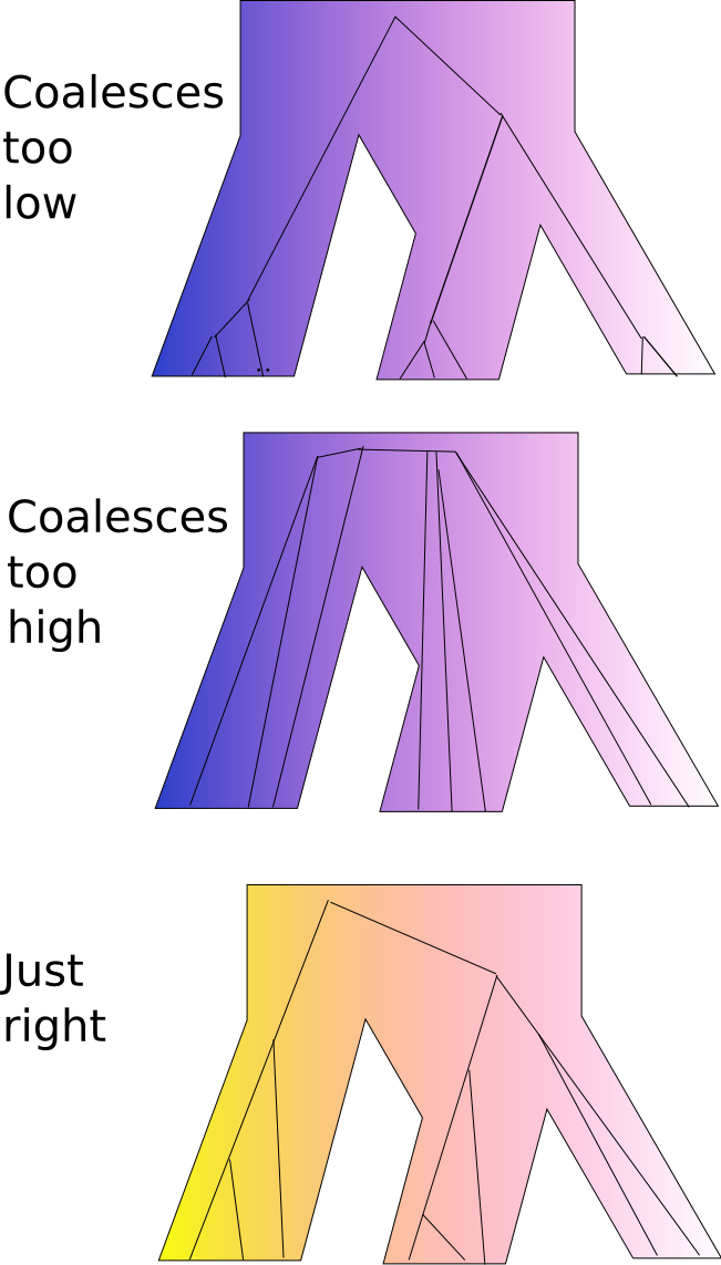
When samples are very closely related, all coalescent events happen very closely to the present time (the sampling time). If so and you look at a branch ending in a species, there is only a single lineage left at the top of the branch. This means we are running in the problem described above; there is no signal in the data left to determine population sizes, and convergence will be difficult. There is no point in adding more sites that have this property, since it would just slow down the calculation without adding more information.

When samples are very distantly related, all coalescent events happen in the branch stemming out of the root. This means, there is no topological information in such samples, and every species tree will fit equally well. On top of this, there is no information to inform population sizes, so SNAPP will not give a lot of information, and will have a terrible time to reach convergence.

In between these extremes, there is the goldilocks zone, where samples coalesc not too early, and not too late, but just in at the right time. In this goldilocks zone, there will be some lineage sorting, so branches above those ending in tips will contain some population size information. This is the kind of data you would like to add.

Of course, it is hard to tell beforehand what kind of data you have, so it is hard to tell beforehand what is the ideal sequence length.


Thanks to David Bryant for pointing out most of the above.

Help, BEAST acts weird! (or how to set up rates) — this site is deprecated: goto https://www.beast2.org/ for up-to-date information

23 June 2015 by Remco Bouckaert

“What is going wrong?” is an often asked question. There can be many things going wrong, but there is one thing that goes wrong more often than other things and it easy to fix.

The first thing you want to check is the settings of the rates in BEAUti. There are two places where rates are set:

  • The site model panel, where the substitution rate is set
  • The clock model panel where the clock rate is set

The final rate used is the product of these rates.

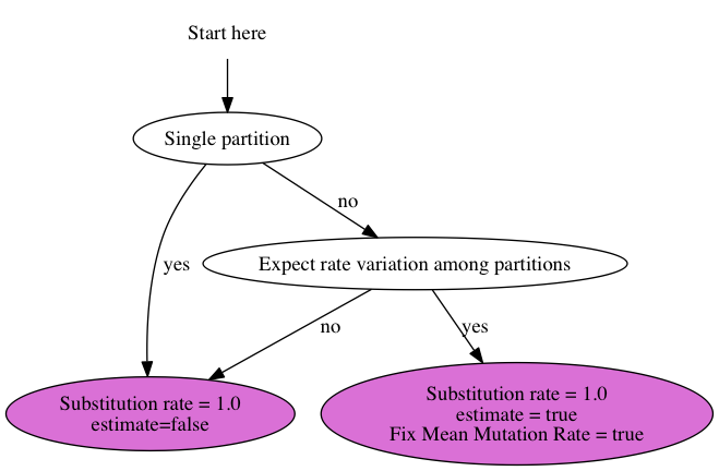
The way to think of the substitution rate is that it is a relative rate with respect to other partitions, while the clock rate is the overall rate for substitutions per site per year (or any other unit of time you choose to use). So, substitution rates will be numbers close to 1, while clock rates tend to be small numbers, such as 4e-9 substitutions per site per year.

Substitution rates

To set up the substitution rates, use this chart:

Standard analysis

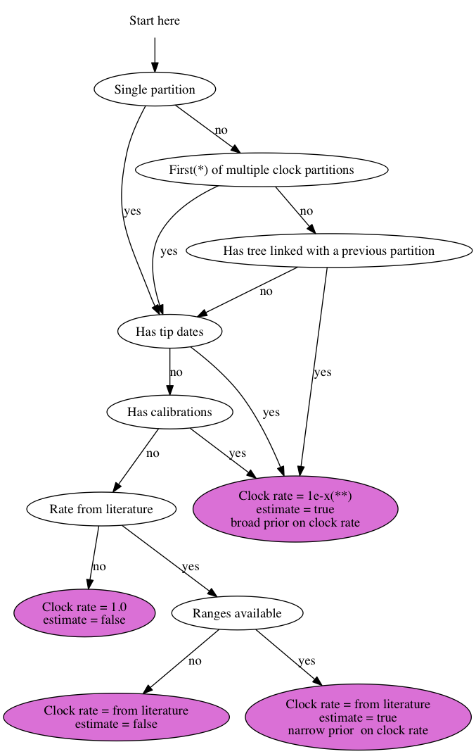
For an analysis using the Standard template, you can go to the clock model tab and use this chart to set up the clock rate:

* Partitions can be ordered arbitrarily. With the first partition I mean the one for which there are either calibrations, tip dates or a rate from the literature, which usually is the first partition listed in the list of clocks, but may be a later one as well.

** Set the clock rate to “1e-x” where x is a number that is somewhere in the region you expect it for your data helps to get through burn-in faster. You could leave it at the default value of 1.0, but it just takes longer to reach convergence. Assuming you are using years as units of time, workable values are 1e-9 for nuclear data, 1e-6 for mitochondrial, bacterial and DNA viral data and 1e-4 for RNA viral data, but if you have more specific information about your sequences it helps to use it to specify starting value.

*BEAST analysis

*BEAST analysis are a bit different in that tip dates are not allowed (at the time of writing) and calibrations are on the species tree, not the gene tree. Usually, all clock rates but the first are estimated using a broad prior. To decide whether the first rate should be estimated or not, use the chart above.

If BEAST still acts weird after rates are set up correctly, just post a question on the BEAST user list.

Better BEAUti templates — this site is deprecated: goto https://www.beast2.org/ for up-to-date information

16 June 2015 by Remco Bouckaert

When developing a BEAUti template, you have to keep in mind that a BEAST model is directed acyclic graph of BEAST objects such as for example shown here. A BEAUti template describes a sub-graph that can be slotted into the overall model. This means the template has to define two things:

  1. A set of BEAST objects
  2. A set of rules on how to put the sub-network into the full graph

Up to now, the rules on how to connect networks to the graph was through BeautiConnector rules specifying the srcID of one of the BEAST objects in the sub-network, and a targetID and inputName specifying which object in the larger network to connect to. Furthermore, connections are not always necessary; if a parameter is kept fixed instead of estimated, there is no need to log it, so there is no need to connect that parameter to any logger. A BeautiConnector only connects conditional on whatever is specified in the if attribute.

Below is a simple template that specifies the HKY substitution model. The BEAST objects are specified in the CDATA section: the HKY substitution model and its kappa parameter and frequencies object, two operators and a prior on kappa. If kappa is estimated (the default) kappa should be connected to the state (see first connector rule). Likewise for frequencies (second rule).


]]>


Scale HKY transition-transversion
parameter of partition s:$(n)


Exchange values of frequencies of partition s:$(n)


HKY transition-transversion
parameter of partition s:$(n)


From BEAST v2.3.0, the connector rules can be integrated in the XML fragment that specify the BEAST objects. At the top level, the target objects are specified through their IDs, and anything that need to be connected can be inserted through nesting these objects. The conditions are encoded in the if attribute in the beauti namespace, so they look like beauti:if followed by the condition. Let’s walk through the example above.

First, we specify the subtemplate header, and the HKY object:


So far nothing different from above. However, next we will connect the kappa and frequency parameter to the state; just define a state element and specify an idref to the state object. The kappa and frequency parameters will be connected to the stateNode input, for which we specify two stateNode elements, and idrefs to the kappa and frequency parameters specified in the HKY block above.


This replaces the first two connector rules in the original template.

Next, we define the prior on kappa. Since it will be connected to the prior, we wrap it in a distribution element with idref to prior. The condition on which to connect (that kappa is in the likelihood and is estimated) is specified in the prior element. We added name="distribution" in order to ensure the prior is connected to the distribution input.


There is another way to specify conditions which is especially handy when there are several items to be connected that are to be connected under the same condition. The if element specified just inside a top-level element in the CDATA block is interpreted as a condition that applies to all of the elements inside. The condition itself is specified in the cond attribute. For example, the operators can be defined like so;


That leaves the connections to the loggers to be defined;


]]>

And that completes the HKY template.

The hope is that this new way for specifying sub-templates is a bit more intuitive once you are used to writing plain BEAST 2 XML. The idea is that going from an example XML to a sub-template just means

  • remove all XML elements outside sub-graph that is not connected to
  • replace all BEAST objects outside the sub-graph with idrefs
  • add conditions (in beauti:if attributes or if elements)

Then the only thing left is to rename IDs so they math partition information and wrap the BEAUti subtemplate bits around the CDATA section.

Sampling tip dates — this site is deprecated: goto https://www.beast2.org/ for up-to-date information

9 June 2015 by Remco Bouckaert

To sample the height of leaf nodes, you need to do the following:

  1. Set up a calibration on the tip you want to sample.
  2. Add an operator for scaling the tip.
  3. Add an entry to the logger if you want to log the leaf height

Tip calibration in BEAUti

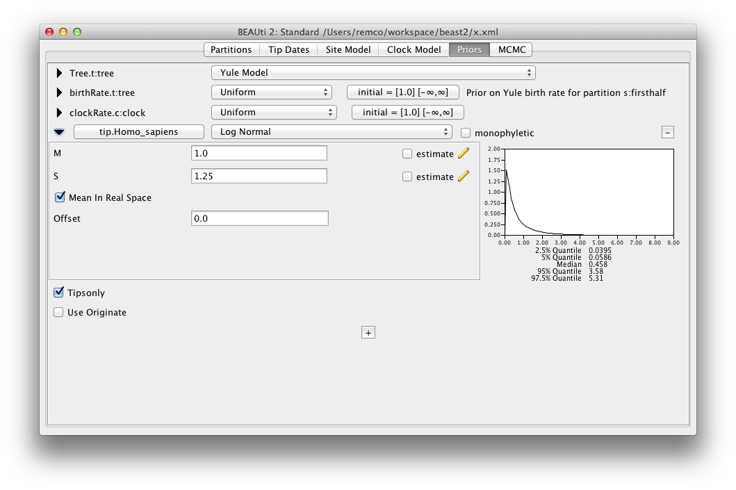
To set up a calibration, the easiest way to do this is by adding a calibration in BEAUti: in the priors panel, hit the little plus (‘+’) button at the bottom of the screen, then specify the leaf you want to sample and give it a unique name. After hitting the OK button, open the details of the prior by pressing the little triangle next to the taxonset (here Homo_sapiens.prior) and a screen shows up like this:

Make sure the Tipsonly box is checked. If you have multiple tips with the same calibration you can put all of these in the same taxonset. With the tipsonly-flag set, the calibration will be applied to the leafs instead of the most recent common ancestor of the set of tips.

Tip calibration in XML

You can also use add an MRCAPrior to the XML inside the distribution element with id=”prior” like so:


Make sure taxon id’s are unique: it is possible a taxon with the id of the tip you want to sample is already specified elsewhere in the XML. If so, when starting BEAST, you will get an error saying something like

Error 104 parsing the xml input file

IDs should be unique. Duplicate id 'Homo_sapiens' found

identifying the id that was already specified.

Also, you want to point to the right tree specified by tree="@Tree.t:tree" in the fragement above.

Tip sample operator in XML

Once the calibration is set up, for each tip you want to sample add an operator to the XML like so:


and edit it as follows:

  • Make sure the id is unique, just changhing the number will do that.
  • The taxonset attribute should refer to the correct taonset.
  • Check that the tree attribute points to the tree you want to sample from. It should be the same tree as in the MRCAPrior.

Add logger entry

To log the leaf height in the trace log, so you can see its mean height, as well as check how well it mixes, add an entry referring to the MRCAPrior to the tracelog. Just place a log entry inside the logger with id=”tracelog” like so:


That’s all.

Species Delimitation with BEAST — this site is deprecated: goto https://www.beast2.org/ for up-to-date information

2 June 2015 by Remco Bouckaert

A few weeks back I attended the conference on Species delimitation in the age of genomics at ANU, which made me realise there is quite an interest in the topic. So, here a quick review of methods for species delimitation available in BEAST. The main methods are

  • Bayes factor delimitation (BFD)
  • Threshold based methods DISSECT/STACEY

Bayes factor delimitation

BFD is based on the multi-species coalescent where there two or more scenarios for species assignments. These scenarios can differ in that taxa for different species can be merged, split or you can even test whether a lineage fits better with one species than another.

The multi-species coalescent can be based on *BEAST or SNAPP, depending on the kind of data that you have: gene sequences for *BEAST and SNP or AFLP data for SNAPP. The idea of BFD is based on a fundamental method of Bayesian methods, which is comparing models based on their marginal likelihoods. Note that this is different from the likelihood typically shown in Tracer; the marginal likelihood is the likelihood marginalised over all parameters in the model.

              prior x likelihood
posterior =  --------------------
              marginal likelihood

The marginal likelihood is most reliably calculated using a stepping stone analysis, though this can be quite tedious to estimate since it is rather computational intensive. There are other methods for model fit, like AICM, that are less computational intensive, but these tend to be less reliable (as outlined by Ayden et al, PloS one, 2014).

For each of the scenarios, you set up a *BEAST or SNAPP analysis with a different species assignment, and estimate the marginal likelihood for each of these scenarios. To do this in BEAST, you need the MODEL_SELECTION package. There are more details here on how to set up a stepping stone/path sampling analysis.

Once you have the marginal likelihoods for each of your scenarios, the Bayes factor comparing say scenario A and B is just the difference between the marginal likelihood estimates.

Threshold based methods DISSECT/STACEY

Threshold based methods are based on setting a level epsilon and declare any split in the species tree that is below that value to be within a species, while any split above the threshold is deemed to represent the birth of a new species. The benefit of this method is that it can be performed during an MCMC run, so it does not require a stepping stone analysis. Also, it does not require setting up different scenarios. However, it does require setting a rather arbitrary threshold, though at the meeting at the ANU conference it was argued by various speakers that defining species is to some extent a social construct, which involves some subjective criteria. So, perhaps this is not such a big deal. update: Graham Jones clarified that the threshold is an approximation to zero without any biological meaning, so should not be interpreted as a social construct but its choice is based on a balance of accuracy and speed.

The DISSECT and STACEY packages allows you to do threshold based species delimitation. STACEY is *BEAST on steroids, with DISSECT as species delimitation method. It integrates out population sizes for the branches, which helps convergence though it means that population size information is lost. Furthermore, it has a number of MCMC proposals that help in mixing; a *BEAST analysis can easily get stuck in an area of tree space that forms a local optimum where the species tree gets locked into a topology because one or more of the gene trees have a good fit to the data preventing the species tree to move to alternative topologies. STACEY offers three extra proposals on top of the standard *BEAST proposals that help to get out of these local optima.

A STACEY analysis can be set up in BEAUti, but DISSECT requires a bit more handwork in editing the XML. For STACEY, you need to select the STACEY template under the File/Templates menu to get started. Both need a bit of fiddling with the XML to get going — see documentation for these packages to work out the details.

After running a DISSECT or STACEY XML file through BEAST, you can use the SpeciesDelimitationAnalyser to process the log files and find out the distribution over species assignments.

Threshold methods have been tested for *BEAST, though should work without too much hassle with SNAPP. The prior for SNAPP needs to be replaced with the

Links

BFD paper for *BEAST.

BFD* paper for SNAPP.

Tutorial for BFD*, with example data.

DISSECT paper, also at bioRxiv.

STACEY info and preprint.